| Issue |
A&A
Volume 549, January 2013
|
|
|---|---|---|
| Article Number | A117 | |
| Number of page(s) | 12 | |
| Section | Stellar atmospheres | |
| DOI | https://doi.org/10.1051/0004-6361/201219868 | |
| Published online | 08 January 2013 | |
- Top
- Abstract
- 1. Introduction
- 2. Observational data and its analysis
- 3. Deriving photospheric surface fluxes by PHOENIX model atmospheres
- 4. Correcting for the photospheric flux in the line cores
- 5. Computation of log R′HK
- 6. Application: deriving the basal chromospheric flux from very large samples
- 7. A new and universal activity index: log
R

- 8. Conclusions and discussion
- Acknowledgments
- References
- List of tables
- List of figures
Ca II H+K fluxes from S-indices of large samples: a reliable and consistent conversion based on PHOENIX model atmospheres
1
Hamburger Sternwarte, Universität Hamburg,
Gojenbergsweg 112,
21029
Hamburg,
Germany
e-mail: This email address is being protected from spambots. You need JavaScript enabled to view it.
2
Departamento de Astronomía, Universidad de
Guanajuato, Apartado Postal
144, 36000
Guanajuato,
Mexico
Received:
22
June
2012
Accepted:
16
November
2012
Abstract
Context. Historic stellar activity data based on chromospheric line emission using O.C. Wilson’s S-index reach back to the 1960ies and represent a very valuable data resource both in terms of quantity and time-coverage. However, these data are not flux-calibrated and are therefore difficult to compare with modern spectroscopy and to relate to quantitative physics.
Aims. In order to make use of the rich archives of Mount Wilson and many other S-index measurements of thousands of main sequence stars, subgiants and giants in terms of physical Ca ii H+K line chromospheric surface fluxes and the related R-index, we seek a new, simple but reliable conversion method of the S-indices. A first application aims to obtain the (empirical) basal chromospheric surface flux to better characterise stars with minimal activity levels.
Methods. We collect 6024 S-indices from six large catalogues from a total of 2530 stars with well-defined parallaxes (as given by the Hipparcos catalogue) in order to distinguish between main sequence stars (2133), subgiants (252) and giants (145), based on their positions in the Hertzsprung-Russell diagram. We use the spectra of a grid of PHOENIX model atmospheres to obtain the photospheric contributions to the S-index. To convert the latter into absolute Ca ii H+K chromospheric line flux, we first derive new, colour-dependent photospheric flux relations for, each, main sequence, subgiant and giant stars, and then obtain the chromospheric flux component. In this process, the PHOENIX models also provide a very reliable scale for the physical surface flux.
Results. For very large samples of main sequence stars, giants and subgiants, we obtain the chromospheric Ca ii H+K line surface fluxes in the colour range of 0.44 < B − V < 1.6 and the related R-indices. We determine and parametrize the lower envelopes, which we find to well coincide with historic work on the basal chromospheric flux. There is good agreement in the apparently simpler cases of inactive giants and subgiants, and distinguishing different luminosity classes proves important. Main sequence stars, surprisingly, show a remarkable lack of inactive chromospheres in the B − V range of 1.1 to 1.5. Finally, we intoduce a new, “pure” and universal activity indicator: a derivative of the R-index based on the non-basal, purely activity-related Ca ii H+K line surface flux, which puts different luminosity classes on the same scale.
Conclusions. The here presented conversion method can be used to directly compare historical S-indices with modern chromospheric Ca ii H+K line flux measurements, in order to derive activity records over long periods of time or to establish the long-term variability of marginally active stars, for example. The numerical simplicity of this conversion allows for its application to very large stellar samples.
Key words: stars: atmospheres / stars: activity / stars: chromospheres / stars: late-type / stars: solar-type
© ESO, 2013
1. Introduction
The study of stellar activity based on the chromospheric Ca ii H+K line emission has a long history: in 1966 O.C. Wilson started a now legendary monitoring program at the Mount Wilson Observatory, which was eventually continued into the 1990ies (Wilson 1978). As a result of these efforts, the so-called Mount Wilson S-index (SMWO-index), a purely empirically determined observational quantity, was established as a standard chromospheric activity indicator for cool stars. A conversion of this empirical SMWO-index into a physical quantity, i.e., a chromospheric emission line surface flux, was introduced by Middelkoop (1982) and Rutten (1984), as well as the related log R′HK-index, which can be derived from the SMWO-index. Soon, the log R′HK-index became the new standard activity indicator. R′HK is the chromospheric flux or “flux excess” in the Ca ii H+K lines, normalised to the bolometric flux (see Linsky et al. 1979).
Many observational studies on stellar chromospheric activity make use of these indices. For
example, in their landmark paper on the rotation-activity connection Noyes et al. (1984) defined a colour-dependent photometric flux
correction for the Ca ii H+K lines and derived a relation between
 and the Rossby number. Schrijver (1987) introduced
the concept of a “basal chromospheric flux” in the context of stellar activity
investigations which used the S-index. In a larger sample of stars the Ca ii H+K
line fluxes show an empirical lower limit, i.e., the already mentioned “basal chromospheric
flux”, which appears not to be of photospheric nature, rather, it reflects the chromospheric
heating of entirely inactive stars, depending sensitively on effective temperature and thus
the B − V-colour (Schrijver 1987; Rutten et al. 1991; Strassmeier et al. 1994). Any dependence on luminosity
class must be very subtle, since it has so far not been resolved (Rutten et al. 1991; Strassmeier et al.
1994).
and the Rossby number. Schrijver (1987) introduced
the concept of a “basal chromospheric flux” in the context of stellar activity
investigations which used the S-index. In a larger sample of stars the Ca ii H+K
line fluxes show an empirical lower limit, i.e., the already mentioned “basal chromospheric
flux”, which appears not to be of photospheric nature, rather, it reflects the chromospheric
heating of entirely inactive stars, depending sensitively on effective temperature and thus
the B − V-colour (Schrijver 1987; Rutten et al. 1991; Strassmeier et al. 1994). Any dependence on luminosity
class must be very subtle, since it has so far not been resolved (Rutten et al. 1991; Strassmeier et al.
1994).
The usefulness of the SMWO-index as a versatile activity indicator thus depends on the possibility to convert it into physical fluxes. By its definition given by O.C. Wilson, S is the ratio between the fluxes in the 1 Å wide cores of the Ca ii H+K lines over two nearby, 20 Å wide segments of pseudo-continua. Since all these components are measured simultaneously, the SMWO-index is insensitive to changes in sky transparency, seeing or transient instrumental effects – very obvious advantages at the time!
The conversion of S-indices into fluxes, (see early work by Middelkoop 1982 and Rutten 1984) relates the signal originally received in in the pseudo-continua of the S-indices to the stellar bolometric flux. Since the Ca ii H+K line core detectors were not designed to measure absolute fluxes (Middelkoop 1982), a conversion between count rates and bolometric flux also had to be derived (cf., Middelkoop 1982), the so-called Ccf-function, which made it possible to convert the observed S-index into absolute surface flux quite easily, yet a number of uncertainties remained, especially by the steep and complex dependence of the conversion on the stellar effective temperature.
Today, it is possible to reliably compute the photospheric surface flux component of the Ca II line cores as well as of the pseudo continua used for the SMWO-index definition. The synthetic spectra used for our work are based on non-LTE PHOENIX model atmospheres (Hauschildt et al. 1999). As a further advantage, any such well-matched model spectrum provides a very good reference scale of the spectral surface flux for each star, as it has been determined from “first principles” rather than by a series of inaccurate calibration steps.
In addition to carefully consider the stellar colour (as an indicator of, mainly, the effective temperature) we here also distinguish between different luminosity classes. This is necessary, because even though the basal flux itself appears to be independent of luminosity class, the SMWO-index is not, since its its photospheric contributions are gravity-sensitive. Hence we classify the stars into main sequence, subgiant and giant objects (luminosity classes V, IV and III), using the parallax measurements by the Hipparcos satellite (Perryman et al. 1992) to derive absolute magnitudes and positions in the empirical Hertzsprung-Russell diagram (thereafter HR-diagram).
As a first application of our improved conversion technique, we here revisit the problem of the basal flux (see Pérez Martínez et al. 2011 for a recent study of this subject). To accomplish this, we first estimate the empirical lower envelopes of the S-indices over B − V, separately for each of the three luminosity classes above, to obtain an empirical minimal S-index. With our new conversion method, we then derive the respective photospheric surface fluxes in the pseudo-continua and the Ca ii H+K lines, and finally we calculate the chromospheric excess flux for each star, which in the cases of minimal S-indices is well consistent with the basal flux.
Considering the resulting minimal or “basal” chromospheric flux as a non-active phenomenon, we finally present a new, “pure” and universal activity indicator, which does not include the basal chromospheric flux. Since it is also purely line-flux-based (unlike the SMWO-index), this new indicator puts the activity of different luminosity classes on the same scale.
2. Observational data and its analysis
2.1. S-index
The Mount Wilson S-index (denoted by SMWO in the following)
has been used for decades as an activity index in the optical spectral range.
SMWO defined as the ratio of counts obtained in a triangular
bandpass with a 1.09 Å FWHM in the centres of the Ca ii H+K lines and two
continua with a width of 20 Å centred at 3901.07 Å and 4001.07 Å, respectively, and
multiplied by some (historical) scaling factor α (Duncan et al. 1991): 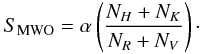 (1)The
factor α is an empirical conversion factor to maintain consistency
between the first and second detector used in the Mount Wilson survey. Many measurements
of S-indices have been carried in the last decades; for this paper we specifically use the
S-indices listed in the catalogues by Duncan et al.
(1991), Henry et al. (1996), Gray et al. (2003, 2006), Wright et al. (2004), and Jenkins et al. (2011). Duncan et al. (1991) report the minimal, maximal and mean
SMWO values for the observed stars collected for those years
when the respective objects were observed, we only use the minimal and maximal values as
reported by Duncan et al. (1991). In the other
catalogues only one SMWO value is reported for the observed
objects.
(1)The
factor α is an empirical conversion factor to maintain consistency
between the first and second detector used in the Mount Wilson survey. Many measurements
of S-indices have been carried in the last decades; for this paper we specifically use the
S-indices listed in the catalogues by Duncan et al.
(1991), Henry et al. (1996), Gray et al. (2003, 2006), Wright et al. (2004), and Jenkins et al. (2011). Duncan et al. (1991) report the minimal, maximal and mean
SMWO values for the observed stars collected for those years
when the respective objects were observed, we only use the minimal and maximal values as
reported by Duncan et al. (1991). In the other
catalogues only one SMWO value is reported for the observed
objects.
2.2. Distinction by luminosity class
We matched all stars with available SMWO-data with entries in the Hipparcos catalogue (Perryman & ESA 1997) and rejected all objects without appropriate parallaxes and corresponding B − V data. The thus obtained total number of stars and S-index measurements is 4489 and 9913, respectively. Using the Hipparcos parallaxes the absolute magnitudes of the stars can be calculated and thus their position in the HR-diagram be determined. In order to define the luminosity class of the stars we use the average absolute magnitudes of main sequence, subgiant, giant and bright giant stars as listed by Allen (1973). For the average absolute magnitudes of subgiant stars we assumed a value of +3 mag to apply also for all colours B − V > 1.2; this assumption is necessary for the definition of the boundaries of the luminosity class of main sequence stars with a colour index B − V > 1.2. To define the luminosity class we computed the absolute magnitude difference between neighbouring luminosity classes as a function of colour and defined a width Δ(M) of 20%. This value of Δ(M) was used to define the lower and upper boundary of the absolute magnitude area for the luminosity classes.
For main sequence stars the Δ(M)-values of the difference between the absolute magnitude of main sequence and subgiant stars are used for the definition of the lower and upper boundary. For the other luminosity classes, the lower boundary is defined by the Δ(M) of difference between the absolute magnitude of this class and the darker class. The upper boundary is defined by the Δ(M) of difference between the absolute magnitude of this class and the brighter class. Only stars located in this magnitude range are used. All stars that could not be uniquely attributed to a luminosity class were rejected and are not used for subsequent analysis; in this fashion we selected a total of 2530 stars with 6024 S-index measurements, i.e., 2133 main sequence stars with 4950 S-indices, 252 subgiants with 836 S-indices and 145 giant stars with 238 S-indices. An HR-diagram with the selected stars is shown in Fig. 1.
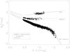 |
Fig. 1 HR-diagram of selected sample stars. The solid lines are the average absolute magnitudes of main sequence, subgiant and giant stars as listed by Allen (1973). |
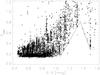 |
Fig. 2 SMWO (below 1.2) vs. B − V colour for selected main sequence stars; the derived lower envelope is drawn with a solid line, the uncertainty of 0.02 indicated by the dashed line. |
 |
Fig. 3 SMWO (below 0.25) vs. B − V colour for selected subgiant stars; the derived lower envelope is drawn with a solid line, the uncertainty of 0.02 indicated by the dashed line. |
2.3. Minimal S-indices
In Figs. 2–4 we show SMWO vs. B − V colour for the finally selected sample stars in the different luminosity classes. An inspection of Figs. 2−4 shows clearly defined lower edges for the observed S-index distributions. To numerically construct a functional form describing this lower edge we proceeded as follows: For the main sequence stars we adopted a constant S-index in the range 0.44 ≤ B − V < 0.94, a linear increase in the range 0.94 ≤ B − V < 1.06 and 1.06 ≤ B − V < 1.35, and a linear decrease in the range 1.35 ≤ B − V < 1.50, and for 1.5 ≤ B − V again a constant value was adopted, but the actual number of measurements in this range is very small. For the subgiant stars we used two linear dependences split at B − V = 0.55, and for the giants only a single B − V range. To obtain the lower envelopes, the edge slopes are modelled with a polynomial of order 0 or 1 and adjusted so that at 99% of S-indices lie above the edge curve, for B − V > 1.50 for the main sequence stars and giant stars only ≈ 98% of the data are above the fit. The estimated parameters for the envelopes of the SMWO distributions for the various B − V ranges and luminosity classes are provided in Table 1.
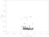 |
Fig. 4 SMWO vs. B − V colour for selected giants; the derived lower envelope is drawn with a solid line, the uncertainty of 0.02 indicated by the dashed line. |
In this context it must be kept in mind that the catalogued S-index data have been collected from different sources with different internal accuracies of the reported SMWO-values. The main uncertainty of the SMWO-values is the transformation from the internal S-index of the different surveys into the SMWO with the trivial exception of the catalogue by Duncan et al. (1991). To evaluate this transformation uncertainty, the objects of the single catalogues were matched with Duncan et al. (1991) and the SMWO-values for those objects, observed in both surveys and with ⟨ SMWO ⟩ < 0.2, were compared. The standard deviations of the residuals were calculated for each survey comparison. The average standard deviation was found to be 0.020 ± 0.003 and was assumed to be the uncertainty of the transformation in general. This uncertainty is clearly an upper limit for the transformation error because in the process all objects were included irrespective of their actual activity levels. Gray et al. (2003) quote the error of SMWO with ± 0.01 so that the real transformation error is probably between 0.01 to 0.02.
Coefficients of the equation min SMWO = a + b(B − V) for the envelope of the S-Index.
In Figs. 2–4, the lower envelopes reduced by a transformation error of 0.02 are plotted as dashed lines. For the subgiant and giant stars all data points are located above these dashed lines, while for the main sequence stars five S-index values are below the dashed lines.
In the following, we discuss these data points individually. The first data point refers to one measurement of HIP 64345 with a B − V value of 0.622; Duncan et al. (1991) lists three single measurements of HIP 64345 with SMWO = 0.120, 0.154, 0.195 respectively with an average value is 0.156 ± 0.022, thus HIP 64345 is certainly not always near the lower envelope. The second data point refers to HIP 51263 with a B − V value of 1.170, observed once by Gray et al. (2006) with SMWO = 0.212. The third data point below the dashed line refers to the star HIP 12493 with a B − V value of 1.185 and denotes one of two S-indices listed by Duncan et al. (1991) as 0.401 and 0.418 respectively. The fourth data point in the B − V range of 1.06 to 1.35 belongs to HIP 17749 with a B − V value of 1.314; Gray et al. (2003) report a SMWO-value of 0.559, while Duncan et al. (1991) lists a minimal and maximal SMWO-value of 0.724 and 0.832, respectively. Obviously the values between Gray et al. (2003) and Duncan et al. (1991) differ significantly. Finally, the fifth S-index below the dashed line refers to HIP 54035 with B − V = 1.502. Duncan et al. (1991) reports a SMWO of 0.188, which is the minimum out of 9 observations taken in 1979. On the other hand, the average minimal S-index of HIP 54035 from 16 years of observations is 0.343 with a standard deviation of 0.051 (Duncan et al. 1991), we therefore consider the low value of 0.188 as an outlier.
3. Deriving photospheric surface fluxes by PHOENIX model atmospheres
The SMWO-index can also be described with the stellar surface
fluxes emitted in the Ca ii H+K lines (Middelkoop
1982; Rutten 1984). Middelkoop (1982) expressed the S-index in terms of  (2)where
ℱHK is the stellar surface flux in the Ca ii lines, ℱRV the
surface flux in both continua and the factor α is a historical,
dimensionless conversion factor (discussed in detail by Hall
et al. 2007). Following Hall et al. (2007)
we use the value α ~ 19.2 to convert ℱRV into an
absolute surface flux in the Ca ii lines according to the measured S-indices.
According to this relation a conversion of S-indices into chromospheric surface fluxes must
thus be done in two steps: first, the continuum fluxes ℱRV are derived for
different B − V values from synthetic spectra computed in
NLTE with the multi-purpose stellar atmosphere code PHOENIX (Hauschildt et al. 1999, see below). This defines the denominator of the
SMWO. Second, the photospheric flux components of the line
cores must be computed in the same way and corrected for (see next section).
(2)where
ℱHK is the stellar surface flux in the Ca ii lines, ℱRV the
surface flux in both continua and the factor α is a historical,
dimensionless conversion factor (discussed in detail by Hall
et al. 2007). Following Hall et al. (2007)
we use the value α ~ 19.2 to convert ℱRV into an
absolute surface flux in the Ca ii lines according to the measured S-indices.
According to this relation a conversion of S-indices into chromospheric surface fluxes must
thus be done in two steps: first, the continuum fluxes ℱRV are derived for
different B − V values from synthetic spectra computed in
NLTE with the multi-purpose stellar atmosphere code PHOENIX (Hauschildt et al. 1999, see below). This defines the denominator of the
SMWO. Second, the photospheric flux components of the line
cores must be computed in the same way and corrected for (see next section).
3.1. Synthetic spectra
Using the PHOENIX code to compute a grid of model atmospheres, we obtain the basis for
the above conversion of S-indices into fluxes, using a representative grid of stellar
parameters. Input parameters are Teff,
M/M⊙ and log g as
well as the metallicity and rotational velocity. The effective temperature
Teff is related to the measured colour index
B − V (Gray
2005) through  (3)For
main sequence stars values for M and log g are used
from Gray (2005, Table B.1), while the masses
M for the giant stars are calculated from the values of
R and log g as taken from Gray (2005, Table B.2).
(3)For
main sequence stars values for M and log g are used
from Gray (2005, Table B.1), while the masses
M for the giant stars are calculated from the values of
R and log g as taken from Gray (2005, Table B.2).
Adopted stellar parameters.
For subgiants the stellar parameter M and log g are
derived from Allende Prieto & Lambert
(1999). Average vsini-values for main sequence
and giant stars are taken from Gray (2005, Tables B.1
and B.2) and have been evaluated through  For
subgiants v sini-values were estimated from Schrijver & Pols (1993) in the relevant
B − V range.
For
subgiants v sini-values were estimated from Schrijver & Pols (1993) in the relevant
B − V range.
For all synthetic spectra, solar metallicity and a microturbulence velocity of 2.0 km s-1 were used. A summary of all stellar parameters used for the spectrum calculation, as well as the vsini-values used for velocity broadening is summarized in Table 2.
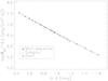 |
Fig. 5 log (ℱRV/19.2 in the Ca ii R+V band passes, calculated from the synthetic spectra, vs. the colour index B − V for main sequence, subgiant and giant stars. |
3.2. The flux in the pseudo-continua, ℱRV as a function of stellar colour
From the synthetic spectra the computed spectral surface flux is integrated in the two
S-index continuum band passes. In Fig. 5 the surface
flux in these continuum band passes (divided by 19.2) is shown for main sequence, subgiant
and giant stars, respectively as a function of B − V
colour. As is obvious from Fig. 5, the logarithm of
the continuum flux ℱRV/19.2 shows a clearly defined linear dependence on the
colour index B − V. Furthermore, flux trends are very
similar for the main sequence and subgiant stars. Hence we can use a single flux relation
for both, main sequence and subgiant stars: 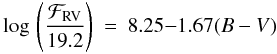 (4)for
main sequence stars (0.44 ≤ B − V ≤ 1.6) and subgiant
stars (0.44 ≤ B − V ≤ 1.1), while we obtain the relation
(4)for
main sequence stars (0.44 ≤ B − V ≤ 1.6) and subgiant
stars (0.44 ≤ B − V ≤ 1.1), while we obtain the relation
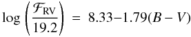 (5)for
giant stars (0.76 ≤ B − V ≤ 1.18). The standard
deviations of the fit residuals are 0.016 for Eq. (4) and 0.008 for Eq. (5),
respectively. The reason for difference between the flux relations are caused by gravity
effects. Using the relations Eqs. (4)
or (5) and (2), the (absolute) flux in the Ca ii H+K lines can now be
easily calculated from the observed B − V colour and the
SMWO-index.
(5)for
giant stars (0.76 ≤ B − V ≤ 1.18). The standard
deviations of the fit residuals are 0.016 for Eq. (4) and 0.008 for Eq. (5),
respectively. The reason for difference between the flux relations are caused by gravity
effects. Using the relations Eqs. (4)
or (5) and (2), the (absolute) flux in the Ca ii H+K lines can now be
easily calculated from the observed B − V colour and the
SMWO-index.
3.3. Comparison with classical methods
Next we compare our new relations to convert the S-index into an absolute surface flux to
the classical method derived by Middelkoop (1982)
and Rutten (1984). In the classical method as
derived by Middelkoop (1982) and Rutten (1984) the continuum flux (in arbitrary flux
units) can be expressed as 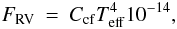 (6)using
the stars effective temperature Teff and a colour-dependent
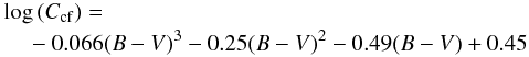
correction factor Ccf defined through (Rutten 1984)
(6)using
the stars effective temperature Teff and a colour-dependent
correction factor Ccf defined through (Rutten 1984)  (7)for main sequence
stars in the range 0.3 ≤ B − V ≤ 1.6, and through
(7)for main sequence
stars in the range 0.3 ≤ B − V ≤ 1.6, and through
 (8)for
sub- and giant stars in the range 0.3 ≤ B − V ≤ 1.7.
Similarly, Rutten (1984) expresses the relative
flux FHK as a function of SMWO
through
(8)for
sub- and giant stars in the range 0.3 ≤ B − V ≤ 1.7.
Similarly, Rutten (1984) expresses the relative
flux FHK as a function of SMWO
through 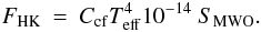 (9)Finally,
the relative surface fluxes are converted into absolute surface fluxes by multiplication
with a constant K (Middelkoop
1982; and Rutten 1984)
(9)Finally,
the relative surface fluxes are converted into absolute surface fluxes by multiplication
with a constant K (Middelkoop
1982; and Rutten 1984) 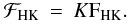 (10)Middelkoop (1982) and Rutten (1984) used differed methods to obtain this conversion factor
K. Rutten (1984) used the
absolute surface flux and a mean S-index of the Sun to obtain the conversion factor
K, while Middelkoop (1982) used
the Ca ii H+K line flux calibration by Linsky
et al. (1979), who, however, did not use the HKP Ca ii H+K line
bandpass, but rather a rectangle bandpass with the Ca ii H(1) minima and K(1)
minima points as boundaries. At any rate, the constant K does depend on
the bandpass in which solar ℱHK-values are determined, and a more recent
determination of K by Hall et al.
(2007) yields a K value of
(0.95 ± 0.11) × 106 erg cm-2 s-1 for a 1 Å
rectangular bandpass; a list of different K values and a more detailed
discussion of the classical conversion of the S-index into the ℱHK is provided
in the same paper.
(10)Middelkoop (1982) and Rutten (1984) used differed methods to obtain this conversion factor
K. Rutten (1984) used the
absolute surface flux and a mean S-index of the Sun to obtain the conversion factor
K, while Middelkoop (1982) used
the Ca ii H+K line flux calibration by Linsky
et al. (1979), who, however, did not use the HKP Ca ii H+K line
bandpass, but rather a rectangle bandpass with the Ca ii H(1) minima and K(1)
minima points as boundaries. At any rate, the constant K does depend on
the bandpass in which solar ℱHK-values are determined, and a more recent
determination of K by Hall et al.
(2007) yields a K value of
(0.95 ± 0.11) × 106 erg cm-2 s-1 for a 1 Å
rectangular bandpass; a list of different K values and a more detailed
discussion of the classical conversion of the S-index into the ℱHK is provided
in the same paper.
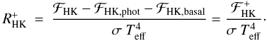
In order to compare the classical method for the calculation of ℱHK with our new method, we computed the ℱHK-values both classically and with our new method. For the classical method, we used a value of K = (1.07 ± 0.13) × 106 erg cm-2 s-1 as derived by Hall et al. (2007) for a triangular bandpass with a 1.09 Å FWHM in the centres of the Ca ii H+K lines. In Fig. 6 we show this comparison for our sample main sequence stars. An inspection of Fig. 7 shows that the flux with the new flux calculation method in general yields somewhat larger values than the flux calculated with the classical method. For F and G type stars the ℱHK-values are very similar, the larger values are found for the later-type stars.
 |
Fig. 6 Logarithm of ℱHK (calculated with Eqs. (2) and (4)) vs. logarithm of classical ℱHK (calculated with Eq. (10)) for the main sequence stars; solid line indicates equality. |
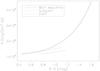 |
Fig. 7 The “constant” K vs. B − V colour. |
Next we compared the classical relation with our new relations. In the classical method
the factor K is assumed to be colour independent. In our approach one
immediately notices that this is not the case if one compare the relations. Writing
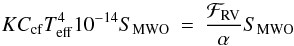 we
deduce
we
deduce 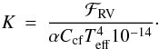 (11)Since
in Eq. (11)
Teff, ℱRV and Ccf all
depend on colour, K will also depend on colour. Using
α = 19.2 and the approximations in Eqs. (3), (4) and (7), we obtain expressions for main sequence
stars through
(11)Since
in Eq. (11)
Teff, ℱRV and Ccf all
depend on colour, K will also depend on colour. Using
α = 19.2 and the approximations in Eqs. (3), (4) and (7), we obtain expressions for main sequence
stars through 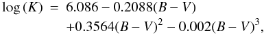 (12)using
Eqs. (3), (4) and (8), for subgiant
stars through
(12)using
Eqs. (3), (4) and (8), for subgiant
stars through  (13)and
using Eqs. (3), (5) and (8), for giants through
(13)and
using Eqs. (3), (5) and (8), for giants through  (14)The
resulting colour dependences are graphically shown in Fig. 7 for the three considered luminosity classes. As is clear from Fig. 7, there is the strong colour dependence for
K with larger B − V values for the
main sequence stars at which the subgiant and giant stars show a linear trend. This
explains the larger ℱHK-values for the later-type stars in our flux conversion.
(14)The
resulting colour dependences are graphically shown in Fig. 7 for the three considered luminosity classes. As is clear from Fig. 7, there is the strong colour dependence for
K with larger B − V values for the
main sequence stars at which the subgiant and giant stars show a linear trend. This
explains the larger ℱHK-values for the later-type stars in our flux conversion.
The colour dependence of K for main sequence stars is caused by the Ccf-values (Eq. (7)), because for derivation of K the same relations for the main sequence and subgiant stars are used without the relation for Ccf. This are differend for the main sequence and subgiant stars.
We next compared our continuum fluxes with the continuum fluxes derived by Linsky et al. (1979). Linsky et al. (1979) used the continuum fluxes in the wavelength range
3925 − 3975 Å for their absolute flux calibration. These absolute continuum fluxes were
based on narrow-band photometry obtained by Willstrop
(1965) and a detailed description of the is given by Linsky et al. (1979), who derived the following the relations:
 (15)
(15) (16)We
note that Linsky et al. (1979) used the colour
index V − R; using Gray
(2005, Table B.1) we can convert these V − R
colours into B − V colours, which we also list in
Table 2. Hence, it is possible to compare very
easily the continuum flux by Linsky et al. (1979)
with our continuum flux. We calculated and graphically compared (see, Fig. 8) the continuum fluxes (Eqs. (15), (16) and (4)) in both colour
ranges. Figure 8 demonstrates a more or less a linear
relation between both continuum fluxes. Computing next the factor K with
the continuum flux by Linsky et al. (1979) and the
relative continuum flux by Rutten (1984) we plot
the logarithm of K vs. B − V colour in
Fig. 9; again a colour dependence in
K appears and for comparison Eq. (4) is also shown in Fig. 9.
Obviously the colour dependences are quite different. This is not unexpected because the
continuum fluxes are different. The deviation from linearity in Fig. 8 and the deviation of the general trend for log K in
Fig. 9 are caused by the non-linearity in the
conversion between B − V and
V − R.
(16)We
note that Linsky et al. (1979) used the colour
index V − R; using Gray
(2005, Table B.1) we can convert these V − R
colours into B − V colours, which we also list in
Table 2. Hence, it is possible to compare very
easily the continuum flux by Linsky et al. (1979)
with our continuum flux. We calculated and graphically compared (see, Fig. 8) the continuum fluxes (Eqs. (15), (16) and (4)) in both colour
ranges. Figure 8 demonstrates a more or less a linear
relation between both continuum fluxes. Computing next the factor K with
the continuum flux by Linsky et al. (1979) and the
relative continuum flux by Rutten (1984) we plot
the logarithm of K vs. B − V colour in
Fig. 9; again a colour dependence in
K appears and for comparison Eq. (4) is also shown in Fig. 9.
Obviously the colour dependences are quite different. This is not unexpected because the
continuum fluxes are different. The deviation from linearity in Fig. 8 and the deviation of the general trend for log K in
Fig. 9 are caused by the non-linearity in the
conversion between B − V and
V − R.
 |
Fig. 8 The logarithm continuum flux by Linsky et al. (1979) vs. the logarithm of our continuum flux and the solid line represents a linear regression |
 |
Fig. 9 Logarithm of K vs. B − V calculated with the our and Linsky et al. (1979) continuum flux |
At any rate, for both continuum flux determination we obtaine a colour dependence of log K. Therefore, we conclude K is colour-dependent if the relative continuum flux by Rutten (1984) is used. The reason for this dependence lies the definition and accuracy of Ccf function. Therefore it is advisable to perform a new definition of the Ccf function. Today, more accurate values for B − V colours, visual magnitude and bolometric corrections are available to define a Ccf function than in the early 1980s.
However, is such a redefinition of the Ccf function really necessary? Our definition of the continuum flux is an alternative to such redefinition of the Ccf function. Furthermore, our relations is in an absolute surface flux scale so that a conversion from a relative surface flux into the absolute surface flux is not necessary and thus the definition of a conversion factor K is not necessary. We consider this as a great advantage over the flux conversion method of Middelkoop (1982) and Rutten (1984). Another advantage is our method simplifies the conversion of the S-index into the absolute surface flux.
Finally, using Eq. (4) we computed ℱHK with equation for the Sun adopting B − V = 0.642 ± 0.004 mag (Cayrel de Strobel 1996) and ⟨ SMWO ⟩ = 0.164 (Wilson 1978) and obtained an absolute surface flux of (2.47 ± 0.10) × 106 erg cm-2 s-1. Comparing this value with ℱHK = (2.172 ± 0.11) × 106 erg cm-2 s-1 as derived by Oranje (1983), our new value is value is ≈14% larger. Oranje (1983) determined the flux in a triangular bandpass with FWHM of 1.09 Å from the Sacramento Peak Observatory (SPO) Solar Atlas with the absolute irradiance data of Thekaekara (1974), who estimated an accuracy of the absolute irradiance data of ±5%. We therefore assume an uncertainty of σℱHK ≈ ±0.11 × 10⁶ erg cm-2 s-1 for their absolute surface flux. To explain the remaining discrepancy, we note that the true solar value of SMWO depends on the actual state of solar activity, and the exact epoch of the SPO Solar Atlas is unknown. Furthermore there may also be errors in the model atmospheric spectra and the used flux relations (cf., Eqs. (4) and (5)). Therefore we conclude that both values are consistent with each other within these uncertainties.
4. Correcting for the photospheric flux in the line cores
In order to obtain the true flux excess in the Ca ii H+K lines (ΔℱHK),
the photospheric flux contribution (ℱHK,phot) in the line centre has to be
subtracted. A B − V colour dependent photospheric
correction was introduced by Noyes et al. (1984)
through  (17)where
RHK,phot is defined as the photosphere flux normalised by the
bolometric flux through
(17)where
RHK,phot is defined as the photosphere flux normalised by the
bolometric flux through  (18)the
effective temperature was computed by Noyes et al.
(1984) using the relation
(18)the
effective temperature was computed by Noyes et al.
(1984) using the relation  (19)In
Noyes et al. (1984), ℱHK,phot does not
denote the full photospheric flux line contribution, but rather only the photospheric line
flux contribution in the HKP line bandpass exterior to the H1 and K1 line points; this
correction is discussed by Hartmann et al. (1984).
(19)In
Noyes et al. (1984), ℱHK,phot does not
denote the full photospheric flux line contribution, but rather only the photospheric line
flux contribution in the HKP line bandpass exterior to the H1 and K1 line points; this
correction is discussed by Hartmann et al. (1984).
Equation (17) is valid only for main sequence stars. Therefore, we derived new ℱHK,phot(B − V) relations separately for main sequence, subgiant and giant stars from our synthetic spectra; for consistency, the same synthetic spectra were used for the derivation of the ℱRV-conversions. To obtain the photospheric flux contribution in the Ca ii H+K lines (ℱHK,phot), the flux of the synthetic spectrum in the Ca ii H+K lines is integrated over the same band passes as the ones used for the Mount Wilson S-index measurements. In Fig. 10 we plot log ℱHK,phot(B − V) in the Ca ii H+K lines calculated from the synthetic spectra versus B − V-colour for main sequence, subgiant and giant stars, each.
 |
Fig. 10 log ℱHK, phot of the Ca ii H+K lines calculated from the synthetic spectra vs. the colour index B − V for main sequence, sub giant and giant stars; the solid lines indicate the derived photospheric flux relations. |
 |
Fig. 11 ℱHK, phot calculated with Eq. (20) and the ℱHK,phot by Noyes et al. (1984) vs. B − V are shown. |
Again we find an approximate linear dependence of
log ℱHK,phot on the colour index
B − V; only for main sequence stars, the slope of the
photospheric flux relation changes at B − V ≈ 1.28,
therefore we use two linear relations for the respective
B − V ranges. The linear fits of
log ℱHK,phot(B − V) are given by the
following equations:  (20)for
main sequence stars in the colour range
0.44 ≤ B − V < 1.28;
(20)for
main sequence stars in the colour range
0.44 ≤ B − V < 1.28;  (21)for
main sequence stars in the colour range
1.28 ≤ B − V < 1.60;
(21)for
main sequence stars in the colour range
1.28 ≤ B − V < 1.60;  (22)for
subgiant stars in the colour range 0.44 ≤ B − V ≤ 1.1, and
(22)for
subgiant stars in the colour range 0.44 ≤ B − V ≤ 1.1, and
 (23)for
giant stars in the colour range 0.76 ≤ B − V ≤ 1.18. The
standard deviations of the residuals are 0.011 for Eq. (20), 0.009 for Eq. (21),
0.009 for Eq. (22) and 0.007 for Eq. (23).
(23)for
giant stars in the colour range 0.76 ≤ B − V ≤ 1.18. The
standard deviations of the residuals are 0.011 for Eq. (20), 0.009 for Eq. (21),
0.009 for Eq. (22) and 0.007 for Eq. (23).
A comparison of the photospheric fluxes computed with our new method compared to those calculated by Noyes et al. (1984) is shown in Fig. 11 (only for main sequence stars). We specifically plot the photospheric fluxes calculated with Eq. (20) (solid line) and those computed using Eqs. (17)–(19). The photospheric fluxes calculated with Eq. (20) are in general larger than the photospheric flux by Noyes et al. (1984) by at least a factor of two (cf., Fig. 11). This leads to smaller excess and eventually basal fluxes; the effect is smallest for stars like the Sun, and becomes much larger for the coolest objects. This discrepancy is caused by the fact that the photospheric flux correction by Noyes et al. (1984) only considers the photospheric flux in the line wings, while our new photospheric flux correction considers the whole flux in the original HK line band passes.
5. Computation of log R′HK
In addition to the SMWO-index the flux-related quantity
log R′HK is also a frequently used stellar activity index.
Linsky et al. (1979) defined
R′HK as
 (24)where
now the chromospheric excess flux (ℱ′HK) of the Ca ii H+K lines is
normalised with respect to the bolometric flux.
(24)where
now the chromospheric excess flux (ℱ′HK) of the Ca ii H+K lines is
normalised with respect to the bolometric flux.
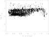 |
Fig. 12 log R′HK-index values of selected sample main sequence stars vs. B − V colour. |
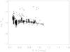 |
Fig. 13 log R′HK-index values of selected sample subgiant stars vs. B − V colour. |
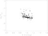 |
Fig. 14 log R′HK-index values of selected giant stars vs. B − V colour. |
The idea behind this normalisation is to compare the activity level of stars with different effective temperatures and B − V colours, respectively. Using our new relations to determine photospheric fluxes and line fluxes, we can now compute new values for log R′HK for all of our sample stars, which we plot in Figs. 12 − 14 for main sequence, subgiant and giant stars in our sample. In Figs. 12 − 14 one recognizes that the lower edges of the log R′HK distributions are different for the main sequence, subgiant and giant stars, respectively; this is not unexpected because the basal flux has not been subtracted. This difference in distribution becomes quite apparent when the log R′HK-data are plotted as histograms (see, Fig. 15) for the respective main sequence, subgiant and giant distributions: The respective distributions are shifted and the lowest activity levels clearly differ for the various luminosity classes.
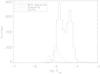 |
Fig. 15 Histogram of log R′HK for the main sequence, subgiant and giant stars |
6. Application: deriving the basal chromospheric flux from very large samples
6.1. Basal flux and stellar colour
The concept of a basal flux was introduced by Schrijver (1987) as that residual flux remaining in the core of the Ca ii H+K lines of inactive stars, once their photospheric line contribution has been removed. Schrijver (1987) was the first to realise that the observed minimum flux levels in the Ca ii H+K lines differed significantly from those expected from a “pure” photosphere and interpreted these fluxes as “basal” chromospheric fluxes, onto which any flux created by magnetic activity is added. Hence, the basal flux is empirically derived from the few stars of almost vanishing magnetic activity, threfore very large stellar samples are needed to empirically delineate this lower activity envelope.
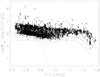 |
Fig. 16 ℱ′HK of selected main sequence stars, lower envelope is indicated with a solid line. The dash-dotted (Rutten 1984) and dotted lines (Rutten et al. 1991) show the basal fluxes one would obtain, if the photospheric contributions are subtracted from the minimal fluxes determined by Rutten in the cited papers. |
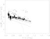 |
Fig. 17 ℱ′HK of selected subgiant stars in the range 0.44 ≤ B − V ≤ 1.11. The data split in two B − V ranges and the lower envelopes are indicated with a solid line. The dashed line shows the basal flux from Strassmeier et al. (1994) (multiplied by a factor 2.5) directly, the dash-dotted (Rutten 1984) and dotted lines (Rutten et al. 1991) show the basal fluxes one would obtain, if the photospheric contributions are subtracted from the minimal fluxes determined by Rutten in the cited papers. |
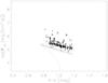 |
Fig. 18 ℱ′HK of selected giant stars in the range 0.76 ≤ B − V < 1.18, the lower envelope is labelled with a solid line. The dashed line shows the basal flux from Strassmeier et al. (1994) (multiplied by the factor 2.5) directly, the dash-dotted (Rutten 1984) and dotted lines (Rutten et al. 1991) show the basal fluxes one would obtain, if the photospheric contributions are subtracted from the minimal fluxes determined by Rutten in the cited papers. |
To obtain the basal fluxes we calculate the ℱ′HK-values for our sample stars with measured S-indices using Eq. (2) and the relations Eqs. (20) − (23). The resulting diagrams in terms of ℱ′HK vs. B − V are shown in Figs. 16 − 18. Similar to the S-index distribution, a relatively clearly defined lower boundary of the distribution appears and can be determined. To describe this lower envelope empirically, we use a piecewise polynomial fit of the order 0, 1 and 2. For the description of the lower envelope of the main sequence stars we require four ranges, for the subgiants two and for the giants only one fit range; for completeness, the respective fit values are listed in Table 3. We used a total of 6024 data points for the lower envelope calculation. Only five stars, i.e., HIP 29860 with SMWO = 0.131, HIP 51263 with SMWO = 0.212 HIP 54035 with SMWO = 0.188, HIP 64345 with SMWO = 0.120 and HIP 71981 with SMWO = 0.126 are located below our envelope curves, obviously an insignificant number showing our conservative approach in defining the empirical basal flux.
Coefficients of the equation log ℱHK,basal = a + b(B − V) + c(B − V)2 for the envelope of the ℱ′HK.
6.2. Comparison with literature values
In the following we compare our basal fluxes to those computed by Rutten (1984), Rutten et al. (1991) and Strassmeier et al. (1994). In Figs. 17 and 18 the basal flux is plotted as dashed line obtained derived by Strassmeier et al. (1994) for subgiant and giant stars; since the flux was derived only for the Ca ii K line. We multiplied Strassmeier’s basal flux by a factor of 2.5 to correct for an offset of his surface flux scale as suggested by Schröder et al. (2012). Fig. 18 shows that the basal flux trend derived by Strassmeier et al. (1994) agrees very well with our basal flux for giant stars. On the other hand, trends clearly differ for the subgiant stars (Fig. 17).
Next we plot the basal fluxes derived by Rutten
(1984) and Rutten et al. (1991) in
Figs. 16 − 18 as dash-dot and dotted lines, respectively. Rutten (1984) defined an envelope for the Ca ii H+K line flux in
arbitrary flux units ( ); he had also
divided the data into main sequence stars (LC V and IV-V) and giant stars (LC II to IV).
To obtain the basal flux in physical units, we need to multiply his fluxes by the
conversion factor K (see Sect. 3.3).
Using the value of
K = (1.07 ± 0.13) × 106 erg cm-2 s-1
as derived by Hall et al. (2007) and considering
the photospheric fluxes using Eqs. (20)
to (23), we find the basal fluxes shown
in Figs. 16 − 18 as dash-dotted lines.
); he had also
divided the data into main sequence stars (LC V and IV-V) and giant stars (LC II to IV).
To obtain the basal flux in physical units, we need to multiply his fluxes by the
conversion factor K (see Sect. 3.3).
Using the value of
K = (1.07 ± 0.13) × 106 erg cm-2 s-1
as derived by Hall et al. (2007) and considering
the photospheric fluxes using Eqs. (20)
to (23), we find the basal fluxes shown
in Figs. 16 − 18 as dash-dotted lines.
Inspecting Fig. 16, the basal flux of Rutten (1984) for main sequence stars is comparable to our basal fluxes for the same class of objects but systematically lower. The same applies for the subgiant stars in the B − V range of 0.44 ≤ B − V < 0.55 and giant stars (see Figs. 17, 18); for the subgiant stars in the B − V range of 0.55 ≤ B − V ≤ 1.1, the trend of his basal flux relation is different from our basal flux trend. In a later paper Rutten et al. (1991) defined a minimal Ca ii H+K line flux in absolute flux units for main sequence, subgiant and giant stars together. As shown in Figs. 16, 18 these basal flux trends differ from our basal flux trends.
The comparison of the different basal fluxes with our flux has shown that individual consideration of each luminosity class is important. Rutten (1984) had divided the data into two luminosity classes; for the main sequence and giant stars the basal flux trend are comparable with our basal flux, while for large B − V range of the subgiant stars, the trend is clearly different. Again, this is caused by not distinguishing between, in this case, subgiant and giant stars.
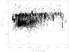 |
Fig. 19
|
Differences in the basal fluxes are also to be expected, because different surface flux calibrations for the Ca ii H+K lines were used. In the case of our basal fluxes, we not only benefit from the extraordinary size of the sample, but also from the reliable flux scale given by the PHOENIX model atmosphere.
An interesting question is why the minimal observed chromospheric flux has a dent between 1.1 ≤ B − V ≤ 1.45. This dent can be also found in the distribution of the original SMWO values, (see Fig. 2). The minimal flux here differs from the B − V trend. This, however, should not matter for the definition of the basal flux, since the dent may simply be caused by the absence of inactive stars in that colour range. Nevertheless, the question remains: what is the reason of such a specific absence? A statistical fluctuation, in any case, is ruled out by the large size of the sample studied here.
7. A new and universal activity index: log
R
An inspection of Fig. 15 shows that the
log R′HK distributions for main sequence, subgiant and
giant stars are different and not comparable with each other. This is not really surprising
since the basal flux has not been subtracted from ℱ′HK. To remedy that situation
we introduce a new, universal and “pure” activity index
 defined by
 (25)Following
the procedures described above we compute for all our
sample stars and plot the results in Figs. 19 − 21; note that five data points are below the basal flux
and hence ℱ′HK becomes negative and an excess flux cannot be meaningfully
defined. We find in general, the values of to be in the
range − 7 to − 3, but note that the lower values are obviously affected by errors both in
the measurements as well as the placement of the basal flux level. In Figs. 19 − 21 a solid line
is plotted at
(25)Following
the procedures described above we compute for all our
sample stars and plot the results in Figs. 19 − 21; note that five data points are below the basal flux
and hence ℱ′HK becomes negative and an excess flux cannot be meaningfully
defined. We find in general, the values of to be in the
range − 7 to − 3, but note that the lower values are obviously affected by errors both in
the measurements as well as the placement of the basal flux level. In Figs. 19 − 21 a solid line
is plotted at  to guide the eye and to
visualise the lower edge of the activity levels. We also note that for main sequence,
subgiant and giant stars, the step at B − V = 0.55 in
for the
subgiant stars (cf., Fig. 11) has disappeared.
to guide the eye and to
visualise the lower edge of the activity levels. We also note that for main sequence,
subgiant and giant stars, the step at B − V = 0.55 in
for the
subgiant stars (cf., Fig. 11) has disappeared.
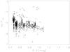 |
Fig. 20
|
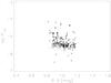 |
Fig. 21
|

 |
Fig. 22 Histogram of |
In Fig. 22 the histograms of the
-distributions
are shown separately for the main sequence, subgiant and giant stars. Compared with the
log R′HK distributions (see Fig. 13) no shifts of the distributions are apparent. In fact, the range of
the distributions of the subgiants and giants is consistent with that of the low-activity
tail of the main sequence star distribution, which of course reaches to far higher activity
levels in log R′HK
Finally, we construct histograms of the distribution
for different B − V-ranges and luminosity classes. In
Fig. 23 we show the
distributions
for main sequence and subgiant stars in the B − V range of
0.44 ≤ B − V < 0.55; a systematic shift of the
towards lower
values is evident for the evolved stars, but there is still a population of comparatively
active subgiants. In the redder B − V ranges (i.e., in
0.55 ≤ B − V < 0.80 shown in Fig. 24 and in
0.80 ≤ B − V ≤ 1.10 in Fig. 25) very few active (sub-)giants remain and the rather bi-modal nature of the
main-sequence distribution becomes apparent.
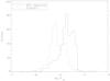 |
Fig. 23 Histogram of |
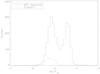 |
Fig. 24 Histogram of |
8. Conclusions and discussion
We have developed a new, numerically simple and reliable method to convert Mt. Wilson S-indices into chromospheric Ca ii surface fluxes, by relations for the photospheric surface flux contributions as functions of the stellar B − V colour index. This has allowed us to study a huge number of S-indices compiled from different literature sources to construct large, meaningful samples, which can be subdivided into luminosity class and B − V colour with sufficient resolution.
As a first application, the empirical lower lower envelopes to these distributions of S-indices and fluxes have been defined to compare with historical work on basal chromospheric flux. For the hotter main sequence stars (B − V < 1.2) and for giant stars, the SMWO-distributions are very well defined, much better than those of the cooler main sequence stars (B − V > 1.2). For late K and M main sequence stars an S-index is difficult to measure because the signal at ≈ 4000 Å is quite low and consequently the number of available data points is small. Other lines than Ca ii K are better suited for activity investigations of these stars.
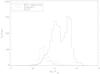 |
Fig. 25 Histogram of |
A significant problem is the uncertainty of the reported S-indices. We chose to transform the measured S-indices into the Mount Wilson system and this transformation is the main uncertainty of the used SMWO. Nevertheless, through the use of different catalogues, the here derived relations for the minimal S-indices and the respective basal fluxes should be quite robust. In principle, we could extend our approach even to study metallicity effects.
With the availability of such a large sample of chromospheric surface fluxes and
well-defined basal fluxes, we find it convenient to propose
as a new,
universal and “pure” activity indicator, which allows a comparison of the activity of stars
in different luminosity classes and of different temperatures on the same scale. The former
is not possible with the classical log R′HK-index. The new
index is a
modification of the latter, where the basal flux is subtracted from ℱ′HK.
We have exploited the availability of large stellar samples, which we can access with our simple but reliable conversion method. The other big advantage and future application is to compare historic activity records of active stars, given as S-indices, with modern monitoring observations based on spectra as by our robotic telescope (González-Pérez et al. 2008). This immediately gives us a time-scale of many decades for a large number of objects monitored then and now, which will help to understand and identify the dynamo processes responsible for so different forms of magnetic activity time-variability as found by the Mt. Wilson monitoring project (Baliunas et al. 1995). Such long time-scales also help to establish the long-term variability or non-variability of marginally active or inactive stars, from which we can learn about the evolution of magnetic activity in evolved stars.
Acknowledgments
This work would have been impossible without the availability of a grid of model atmosphere spectra computed by the PHOENIX code, for which we are most grateful to our colleague P. Hauschildt. We also acknowledge the support through the bilateral (MEX-GER) project Conacyt/DFG No. 147902 and DFG SCHM 1032/36-1.
References
- Allen, C. W. 1973, Astrophysical Quantities, 3rd edn. (University of London: Athlone Press) [Google Scholar]
- Allende Prieto, C., & Lambert, D. L. 1999, A&A, 352, 555 [NASA ADS] [Google Scholar]
- Baliunas, S. L., Donahue, R. A., Soon, W. H., et al. 1995, ApJ, 438, 269 [NASA ADS] [CrossRef] [Google Scholar]
- Cayrel de Strobel, G. 1996, A&ARv, 7, 243 [CrossRef] [Google Scholar]
- Duncan, D. K., Vaughan, A. H., Wilson, O. C., et al. 1991, ApJS, 76, 383 [NASA ADS] [CrossRef] [Google Scholar]
- González-Pérez, J. N., Hempelmann, A., Mittag, M., & Hagen, H.-J. 2008, in SPIE Conf. Ser., 7019 [Google Scholar]
- Gray, D. F. 2005, The Observation and Analysis of Stellar Photospheres, 3rd edn. (Cambridge, UK: Cambridge University Press) [Google Scholar]
- Gray, R. O., Corbally, C. J., Garrison, R. F., McFadden, M. T., & Robinson, P. E. 2003, AJ, 126, 2048 [NASA ADS] [CrossRef] [Google Scholar]
- Gray, R. O., Corbally, C. J., Garrison, R. F., et al. 2006, AJ, 132, 161 [NASA ADS] [CrossRef] [Google Scholar]
- Hall, J. C., Lockwood, G. W., & Skiff, B. A. 2007, AJ, 133, 862 [NASA ADS] [CrossRef] [Google Scholar]
- Hartmann, L., Soderblom, D. R., Noyes, R. W., Burnham, N., & Vaughan, A. H. 1984, ApJ, 276, 254 [NASA ADS] [CrossRef] [Google Scholar]
- Hauschildt, P. H., Allard, F., & Baron, E. 1999, ApJ, 512, 377 [NASA ADS] [CrossRef] [Google Scholar]
- Henry, T. J., Soderblom, D. R., Donahue, R. A., & Baliunas, S. L. 1996, AJ, 111, 439 [NASA ADS] [CrossRef] [Google Scholar]
- Jenkins, J. S., Murgas, F., Rojo, P., et al. 2011, A&A, 531, A8 [NASA ADS] [CrossRef] [EDP Sciences] [Google Scholar]
- Linsky, J. L., McClintock, W., Robertson, R. M., & Worden, S. P. 1979, ApJS, 41, 47 [NASA ADS] [CrossRef] [Google Scholar]
- Middelkoop, F. 1982, A&A, 107, 31 [NASA ADS] [Google Scholar]
- Noyes, R. W., Hartmann, L. W., Baliunas, S. L., Duncan, D. K., & Vaughan, A. H. 1984, ApJ, 279, 763 [NASA ADS] [CrossRef] [Google Scholar]
- Oranje, B. J. 1983, A&A, 124, 43 [NASA ADS] [Google Scholar]
- Pérez Martínez, M. I., Schröder, K.-P., & Cuntz, M. 2011, MNRAS, 414, 418 [NASA ADS] [CrossRef] [Google Scholar]
- Perryman, M. A. C., & ESA 1997, The HIPPARCOS and TYCHO catalogues, Astrometric and photometric star catalogues derived from the ESA HIPPARCOS Space Astrometry Mission, ESA SP, 1200 [Google Scholar]
- Perryman, M. A. C., Hog, E., Kovalevsky, J., et al. 1992, A&A, 258, 1 [NASA ADS] [Google Scholar]
- Rutten, R. G. M. 1984, A&A, 130, 353 [NASA ADS] [Google Scholar]
- Rutten, R. G. M., Schrijver, C. J., Lemmens, A. F. P., & Zwaan, C. 1991, A&A, 252, 203 [NASA ADS] [Google Scholar]
- Schrijver, C. J. 1987, A&A, 172, 111 [NASA ADS] [Google Scholar]
- Schrijver, C. J., & Pols, O. R. 1993, A&A, 278, 51 [Google Scholar]
- Schröder, K.-P., Mittag, M., Pérez Martínez, M. I., Cuntz, M., & Schmitt, J. H. M. M. 2012, A&A, 540, A130 [NASA ADS] [CrossRef] [EDP Sciences] [Google Scholar]
- Strassmeier, K. G., Handler, G., Paunzen, E., & Rauth, M. 1994, A&A, 281, 855 [NASA ADS] [Google Scholar]
- Thekaekara, M. P. 1974, Appl. Opt., 13, 518 [Google Scholar]
- Willstrop, R. V. 1965, MmRAS, 69, 83 [Google Scholar]
- Wilson, O. C. 1978, ApJ, 226, 379 [NASA ADS] [CrossRef] [Google Scholar]
- Wright, J. T., Marcy, G. W., Butler, R. P., & Vogt, S. S. 2004, ApJS, 152, 261 [NASA ADS] [CrossRef] [Google Scholar]
All Tables
Coefficients of the equation min SMWO = a + b(B − V) for the envelope of the S-Index.
Coefficients of the equation log ℱHK,basal = a + b(B − V) + c(B − V)2 for the envelope of the ℱ′HK.
All Figures
|
Fig. 1 HR-diagram of selected sample stars. The solid lines are the average absolute magnitudes of main sequence, subgiant and giant stars as listed by Allen (1973). |
| In the text | |
|
Fig. 2 SMWO (below 1.2) vs. B − V colour for selected main sequence stars; the derived lower envelope is drawn with a solid line, the uncertainty of 0.02 indicated by the dashed line. |
| In the text | |
|
Fig. 3 SMWO (below 0.25) vs. B − V colour for selected subgiant stars; the derived lower envelope is drawn with a solid line, the uncertainty of 0.02 indicated by the dashed line. |
| In the text | |
|
Fig. 4 SMWO vs. B − V colour for selected giants; the derived lower envelope is drawn with a solid line, the uncertainty of 0.02 indicated by the dashed line. |
| In the text | |
|
Fig. 5 log (ℱRV/19.2 in the Ca ii R+V band passes, calculated from the synthetic spectra, vs. the colour index B − V for main sequence, subgiant and giant stars. |
| In the text | |
|
Fig. 6 Logarithm of ℱHK (calculated with Eqs. (2) and (4)) vs. logarithm of classical ℱHK (calculated with Eq. (10)) for the main sequence stars; solid line indicates equality. |
| In the text | |
|
Fig. 7 The “constant” K vs. B − V colour. |
| In the text | |
|
Fig. 8 The logarithm continuum flux by Linsky et al. (1979) vs. the logarithm of our continuum flux and the solid line represents a linear regression |
| In the text | |
|
Fig. 9 Logarithm of K vs. B − V calculated with the our and Linsky et al. (1979) continuum flux |
| In the text | |
|
Fig. 10 log ℱHK, phot of the Ca ii H+K lines calculated from the synthetic spectra vs. the colour index B − V for main sequence, sub giant and giant stars; the solid lines indicate the derived photospheric flux relations. |
| In the text | |
|
Fig. 11 ℱHK, phot calculated with Eq. (20) and the ℱHK,phot by Noyes et al. (1984) vs. B − V are shown. |
| In the text | |
|
Fig. 12 log R′HK-index values of selected sample main sequence stars vs. B − V colour. |
| In the text | |
|
Fig. 13 log R′HK-index values of selected sample subgiant stars vs. B − V colour. |
| In the text | |
|
Fig. 14 log R′HK-index values of selected giant stars vs. B − V colour. |
| In the text | |
|
Fig. 15 Histogram of log R′HK for the main sequence, subgiant and giant stars |
| In the text | |
|
Fig. 16 ℱ′HK of selected main sequence stars, lower envelope is indicated with a solid line. The dash-dotted (Rutten 1984) and dotted lines (Rutten et al. 1991) show the basal fluxes one would obtain, if the photospheric contributions are subtracted from the minimal fluxes determined by Rutten in the cited papers. |
| In the text | |
|
Fig. 17 ℱ′HK of selected subgiant stars in the range 0.44 ≤ B − V ≤ 1.11. The data split in two B − V ranges and the lower envelopes are indicated with a solid line. The dashed line shows the basal flux from Strassmeier et al. (1994) (multiplied by a factor 2.5) directly, the dash-dotted (Rutten 1984) and dotted lines (Rutten et al. 1991) show the basal fluxes one would obtain, if the photospheric contributions are subtracted from the minimal fluxes determined by Rutten in the cited papers. |
| In the text | |
|
Fig. 18 ℱ′HK of selected giant stars in the range 0.76 ≤ B − V < 1.18, the lower envelope is labelled with a solid line. The dashed line shows the basal flux from Strassmeier et al. (1994) (multiplied by the factor 2.5) directly, the dash-dotted (Rutten 1984) and dotted lines (Rutten et al. 1991) show the basal fluxes one would obtain, if the photospheric contributions are subtracted from the minimal fluxes determined by Rutten in the cited papers. |
| In the text | |
|
Fig. 19
|
| In the text | |
|
Fig. 20
|
| In the text | |
|
Fig. 21
|
| In the text | |
|
Fig. 22 Histogram of |
| In the text | |
|
Fig. 23 Histogram of |
| In the text | |
|
Fig. 24 Histogram of |
| In the text | |
|
Fig. 25 Histogram of |
| In the text | |
Current usage metrics show cumulative count of Article Views (full-text article views including HTML views, PDF and ePub downloads, according to the available data) and Abstracts Views on Vision4Press platform.
Data correspond to usage on the plateform after 2015. The current usage metrics is available 48-96 hours after online publication and is updated daily on week days.
Initial download of the metrics may take a while.