| Issue |
A&A
Volume 688, August 2024
|
|
|---|---|---|
| Article Number | A23 | |
| Number of page(s) | 18 | |
| Section | Catalogs and data | |
| DOI | https://doi.org/10.1051/0004-6361/202348988 | |
| Published online | 31 July 2024 | |
Stellar chromospheric activity database of solar-like stars based on the LAMOST Low-Resolution Spectroscopic Survey
II. The bolometric and photospheric calibration★
1
School of Physics and Optoelectronic Engineering, Anhui University,
Hefei
230601,
PR
China
e-mail: This email address is being protected from spambots. You need JavaScript enabled to view it.
2
National Astronomical Observatories, Chinese Academy of Sciences,
Beijing
100101,
PR
China
e-mail: This email address is being protected from spambots. You need JavaScript enabled to view it.
3
University of Chinese Academy of Sciences,
Beijing
100049,
PR
China
4
CAS Key Laboratory of Optical Astronomy, Chinese Academy of Sciences,
Beijing
100101,
PR
China
Received:
18
December
2023
Accepted:
15
May
2024
Abstract
Context. The dependence of stellar magnetic activity on stellar parameters is inspired by the chromospheric activity studies based on the large-scale spectroscopic surveys.
Aims. The main objective of this project is to provide the chromospheric activity parameter database for the LAMOST Low-Resolution Spectroscopic Survey (LRS) spectra of solar-like stars and explore the overall property of stellar chromospheric activity.
Methods. The Ca II H and K lines were employed to construct indicators for assessing and studying the chromospheric activity of solar-like stars. We investigated the widely used bolometric- and photospheric-calibrated chromospheric activity index R′HK, derived from the method in the classic literature (R′HK,classic) and the method based on the PHOENIX model (R′HK,PHOENIX). Since the detailed stellar atmospheric parameters, effective temperature (Teff), surface gravity (log g), and metallicity ([Fe/H]) are available for LAMOST, we estimated the chromospheric activity index R′HK,PHOENIX, along with the corresponding bolometric calibrated index RHK,PHOENIX, taking these parameters into account.
Results. We provided the database of the derived chromospheric activity parameters for 1 122 495 LAMOST LRS spectra of solar-like stars. Our calculations show that log R′HK,PHOENIX is approximately linearly correlated with log R′HK,classic. The results based on our extensive archive support the view that the dynamo mechanism of solar-like stars is generally consistent with the Sun; and the value of the solar chromospheric activity index is located at the midpoint of the solar-like star sample. We further investigated the proportions of solar-like stars with different chromospheric activity levels (very active, active, inactive, and very inactive). The investigation indicates that the occurrence rate of high levels of chromospheric activity is lower among the stars with effective temperatures between 5600 and 5900 K.
Key words: stars: activity / stars: chromospheres
A copy of the catalog is available at the CDS ftp to cdsarc.cds.unistra.fr (130.79.128.5) or via https://cdsarc.cds.unistra.fr/viz-bin/cat/J/A+A/688/A23
© The Authors 2024
 Open Access article, published by EDP Sciences, under the terms of the Creative Commons Attribution License (https://creativecommons.org/licenses/by/4.0), which permits unrestricted use, distribution, and reproduction in any medium, provided the original work is properly cited.
This article is published in open access under the Subscribe to Open model. This email address is being protected from spambots. You need JavaScript enabled to view it. to support open access publication.
1 Introduction
Stellar chromospheric activity, known as the performance of stellar magnetic activity, is expected to reveal the physical mechanism of stars (Hall 2008). The emission in the line cores of Ca II H and K lines is commonly recognized as being sensitive to stellar chromospheric activity. An empirical chromospheric activity index SMWO was introduced to quantify the emission of Ca II H and K lines observed in the Mount Wilson Observatory (MWO) (Wilson 1968; Vaughan et al. 1978). Since SMWO is defined as the ratio between the emission flux in the line cores of Ca II H and K lines and the pseudo-continuum flux (the flux of two 20 Å reference bands in the violet and red sides), it is concise and effective for characterizing the stellar activity cycle (Wilson 1978). However, SMWO is related to the continuum flux, which is governed by the stellar effective temperature (or, equivalently, the color index) (Middelkoop 1982). As a result, it would be inflexible for comparing the emission of Ca II H and K lines among stars of different spectral types.
The ratio between the stellar surface flux in the line core of Ca II H and K lines and the stellar bolometric flux, denoted as RHK, is considered to be marginally affected by the stellar effective temperature (or the color index) and can be derived from SMWO (Linsky et al. 1979; Middelkoop 1982; Rutten 1984). Middelkoop (1982) and Rutten (1984) introduced the bolometric factor Ccf (depends on the color index B − V) and the factor K to convert SMWO to the stellar surface flux in the line cores of Ca II H and K lines. Meanwhile, the photospheric fluxes contained in the line cores of Ca II H and K lines could not be ignored, especially for solar-like stars (Hartmann et al. 1984; Noyes et al. 1984). The photospheric contribution, Rphot, which represents the photospheric flux normalized by the stellar bolometric flux, can analogously be deduced as a function of B − V (Noyes et al. 1984). Subtracting Rphot from RHK, one can derive the widely used bolometric- and photospheric-calibrated chromospheric activity index R′HK.
The R′HK is frequently employed to characterize the relationships between stellar chromospheric activity and other stellar properties such as rotation period (Noyes et al. 1984; Suárez Mascareño et al. 2015; Astudillo-Defru et al. 2017; Brown et al. 2022; Boudreaux et al. 2022) and stellar age (Mamajek & Hillenbrand 2008; Pace 2013; Lorenzo-Oliveira et al. 2018; Booth et al. 2020). The derivation of R′HK may be influenced by the bolometric factor Ccf, the value of K, the photospheric contribution Rphot, and SMWO. Cincunegui et al. (2007) compared the relationship between the Hα line and the Ca II H and K lines, where they recalibrated the Ccf to the range of 0.45 ≤ B − V ≤ 1.81. Suárez Mascareño et al. (2015) and Astudillo-Defru et al. (2017) concentrated on the relationship of R′HK and the rotation period for M dwarfs. Suárez Mascareño et al. (2015) extended the bolometric factor Ccf and the photospheric contribution Rphot to B − V = 1.90 using the empirical spectral library. Astudillo-Defru et al. (2017) derived the equations of Ccf and Rphot based on the empirical and synthetic spectral library, respectively. Lorenzo-Oliveira et al. (2018) and Marvin et al. (2023) provided estimates of Ccf and Rphot as functions of effective temperature.
The stellar surface flux now is relatively accurately determined in synthetic spectral models such as ATLAS, PHOENIX, and MARCS (Munari et al. 2005; Allard & Hauschildt 1995; Gustafsson et al. 2008). The synthetic spectral library PHOENIX was widely used in the calculation of the chromospheric activity index based on the Ca II H and K lines, for example, Mittag et al. (2013) estimated the stellar surface flux as a formula of B − V, and Marvin et al. (2023) derived the relationship between Ccf and the stellar effective temperature. Pérez Martínez et al. (2014) directly cross-matched each observed spectrum with the synthetic spectral library PHOENIX to derive an empirical chromospheric basal flux line. In addition, the PHOENIX spectral library is also used to deduce the photospheric contribution (e.g., Mittag et al. 2013; Astudillo-Defru et al. 2017; Marvin et al. 2023). Astudillo-Defru et al. (2017) pointed out that the photospheric contribution derived from the PHOENIX library is higher than that obtained from empirical spectra by Noyes et al. (1984).
With the development of large-scale photometric and spectroscopic surveys, statistical investigation of stellar chromosphere may disclose some novel phenomena (de Grijs & Kamath 2021). The Large Sky Area Multi-Object Fiber Spectroscopic Telescope (LAMOST, also named the Guoshoujing Telescope) has released massive spectral data since its pilot survey started in 2011 (Cui et al. 2012; Zhao et al. 2012; Luo et al. 2012). The spectra released by the Low-Resolution Spectroscopic Survey (LRS) of LAMOST cover the wavelength from 3700 to 9100 Å with a spectral resolving power (R = λ/Δλ) of about 1800 (Zhao et al. 2012). A number of investigations of chromospheric activity have profited from the several spectral lines recorded by LAMOST, such as the Ca II H and K lines, the Hα line and the Ca II infrared triplet (IRT) lines (e.g., Zhang et al. 2019, 2020; Bai et al. 2021; Han et al. 2023; He et al. 2023; Huang et al. 2024). In our previous work (Zhang et al. 2022, hereafter Paper I), we investigated the Ca II H and K lines of LAMOST LRS spectra and provided a stellar chromospheric activity database; notably, we calibrated the S index value of LAMOST to the scale of MWO. We dedicated this work to describing the chromospheric activity of solar-like stars based on the bolometric-and photospheric-calibrated indexes of LAMOST LRS spectra (He et al. 2021).
This paper is organized as follows. In Sec. 2, we describe the spectral data used in this work. In Sec. 3, the detailed procedures of deriving the chromospheric activity indexes and their uncertainties are illustrated. In Sec. 4, we present the database provided in this work and discuss the chromospheric activity based on the database. Finally, we provide a brief summary and conclusion of this work in Sec. 5.
2 Data collection of solar-like stars
We used the LAMOST LRS spectra in the Data Release 8 (DR8) v2.01, which were observed between October 2011 and May 2020. The LAMOST DR8 v2.0 comprises 10633 515 LRS spectra, among which 6684413 spectra with determined stellar parameters were published in the LAMOST LRS Stellar Parameter Catalog of A, F, G, and K Stars (hereafter referred to as the LAMOST LRS AFGK Catalog). The stellar parameters such as effective temperature (Teff), surface gravity (log g), metallicity ([Fe/H]), heliocentric radial velocity (Vr), and their corresponding uncertainties are provided by the LAMOST Stellar Parameter Pipeline (LASP) (Luo et al. 2015).
We selected the spectra of solar-like stars (Cayrel de Strobel 1996) according to the effective temperatures around the Sun (Teff,⊙ = 5777 K, adopted as in Ramírez et al. 2012) that are in the range of 4800 ≤ Teff ≤ 6300 K, and the metallicities around the Sun ([Fe/H]⊙ = 0.0 dex) that are in the range of −1.0 < [Fe/H] < 1.0 dex. The spectra of main-sequence stars are empirically separated from the giant sample by the criterion of log g as adopted in Paper I:
![Mathematical equation: $\[\log g \geq 5.98{-}0.00035 \times T_{\text {eff }}.\]$](/articles/aa/full_html/2024/08/aa48988-23/aa48988-23-eq1.png) (1)
(1)
The uncertainties of the chromospheric activity indexes are related to the uncertainties of the spectral fluxes and the corresponding stellar parameters derived from the LRS spectra, which are predominantly impacted by the signal-to-noise-ratio (S/N) parameters of LRS spectra. The precision of spectral fluxes of Ca II H and K lines and stellar parameters is primarily affected by the S/N in the g and r bands of LRS. Therefore, the high-S/N spectra of solar-like stars are screened out by the S/N threshold S/Ng ≥ 50.00 and S/Nr ≥ 71.43, as adopted in Paper I. A total of 1 149 216 spectra of solar-like stars are picked out from the LAMOST LRS AFGK Catalog. The band of Ca II H and K lines used to derive the chromospheric activity index refer to the vacuum wavelength range of 3892.17–4012.20 Å (see Paper I). The spectra in this band with zero or negative flux are discarded. We eventually analyzed the chromospheric activity based on 1 122 495 LAMOST LRS spectra of solar-like stars. The distribution of the selected spectral samples is shown in Fig. 1, where the gray dots represent the samples in LAMOST LRS AFGK Catalog. Since abundant stellar information is available in Gaia DR3 (Gaia Collaboration 2023), we identified 861 505 solar-like stars in the selected spectra with gaia_source_id obtainable in LAMOST LRS AFGK Catalog. Given that the LAMOST is dedicated to the spectral survey of large sky areas, 81% of the solar-like stars have been observed only once. Figure 2 displays the histogram of the observation numbers for 861 505 solar-like stars.
In Fig. 3, we show the histograms of the Teff, log g, [Fe/H], and Vr for the 861 505 solar-like stars used in this work. If one star is observed more than once, the values of Teff, log g, [Fe/H], and Vr are taken as the median of the corresponding values of the multiple observed spectra. As illustrated in the LAMOST DR8 release note2, the uncertainties of Teff, log g, [Fe/H], and Vr are relatively high for S/Nr under 30 and are relatively accurate for S/Nr greater than 50. Based on our aforementioned S/N threshold of spectral selection (S/Ng ≥ 50.00 and S/Nr ≥ 71.43), the uncertainties of Teff, log g, [Fe/H], and Vr for the selected stars, which are provided by LASP, are approximately distributed around 25 K, 0.035 dex, 0.025 dex, and 3.5 km s−1, respectively. The LAMOST DR8 release note also provides the parameter comparisons between LAMOST DR8 v2.0 LRS and DR16 (Ahumada et al. 2020) of the Sloan Digital Sky Survey (York et al. 2000). Since the effective temperature plays an important role in Sect. 3, we compare the Teff provided by LASP with the results of Amard et al. (2020) in Appendix A.
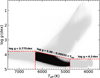 |
Fig. 1 Distribution of selected spectral samples (black dots) of solar-like stars and the samples in LAMOST LRS AFGK Catalog (gray dots) with Teff in the range of 3500 to 7500 K. The vertical and horizontal red lines represent the empirical selection ranges of Teff and log g, respectively; the diagonal red line denotes the corresponding empirical formula in Eq. (1). |
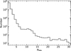 |
Fig. 2 Histogram of number of observations for 861 505 solar-like stars. |
3 Evaluation of the chromospheric activity index of solar-like stars
The following steps are taken in the derivation of the chromospheric activity index R′HK of solar-like stars based on the Ca II H and K lines of LAMOST LRS: (1) definition of SMWO for LAMOST LRS; (2) conversion of SMWO to RHK; (3) derivation of the bolometric- and photospheric-calibrated chromospheric activity index R′HK; (4) estimation of the uncertainty of chromospheric activity indexes.
3.1 Definition of SMWO for LAMOST LRS
The stellar chromospheric activity index has been widely studied and broadened based on the emission of the Ca II H and K lines (e.g., Wilson 1968; Vaughan et al. 1978; Duncan et al. 1991; Baliunas et al. 1995; Hall et al. 2007; Egeland et al. 2017; Boro Saikia et al. 2018). In 1966, the two-channel HKP-1 spectrophotometer was employed at the Mount Wilson Observatory to monitor the emission of stellar Ca II H and K lines (Wilson 1968; Hall et al. 2007). One channel was used to collect data in the 25 Å rectangular bands located on the red and violet sides of the Ca II H and K lines. The counts in the reference bands of this channel were noted as NRV. The other channel was used to measure the emission in the 1 Å rectangular bands centered at Ca II H or K lines. After completing the counts in either H or K lines, the relative instrumental fluxes ![Mathematical equation: $\[F_{\mathcal{H}}=N_{\mathcal{H}} / N_{\mathcal{R} V}\]$](/articles/aa/full_html/2024/08/aa48988-23/aa48988-23-eq2.png) or
or ![Mathematical equation: $\[F_{\mathcal{K}}=N_{\mathcal{K}} / N_{\mathcal{R} V}\]$](/articles/aa/full_html/2024/08/aa48988-23/aa48988-23-eq3.png) could be collected, where N
could be collected, where N![Mathematical equation: $\[\mathcal{H}\]$](/articles/aa/full_html/2024/08/aa48988-23/aa48988-23-eq4.png) and N
and N![Mathematical equation: $\[\mathcal{K}\]$](/articles/aa/full_html/2024/08/aa48988-23/aa48988-23-eq5.png) are the counts in the 1 Å rectangular bands centered at Ca II H and K lines. Wilson (1968) employed
are the counts in the 1 Å rectangular bands centered at Ca II H and K lines. Wilson (1968) employed ![Mathematical equation: $\[F=\frac{1}{2}\left(F_{\mathcal{H}}+F_{\mathcal{K}}\right)\]$](/articles/aa/full_html/2024/08/aa48988-23/aa48988-23-eq6.png) to assess the emission of Ca II H and K lines collected by the HKP-1.
to assess the emission of Ca II H and K lines collected by the HKP-1.
In view of the instrumental effects and certain limitations in the HKP-1, Vaughan et al. (1978) introduced the HKP-2, a four-channel spectrophotometer, in 1977. The H and K channels collected the two 1.09 Å full width at half maximum (FWHM) triangular band passes in the line cores of Ca II H and K lines centered in the air wavelengths of 3968.47 and 3933.66 Å, respectively. In addition, the R and V channels measured the two 20 Å rectangular band passes on the red and violet sides of the Ca II H and K lines (the wavelength ranges in the air being 3991.07–4011.07 Å and 3891.07–3911.07 Å, respectively). The H, K, R, and V channels are exposed sequentially and rapidly, with the exposure time of the H and K channels being eight times that of the R and V channels. To align the HKP-2 data with the HKP-1 data, Vaughan et al. (1978) performed a calibration of the HKP-2 data to match the HKP-1 data by
![Mathematical equation: $\[S_{\mathrm{MWO}}=\alpha \cdot \frac{N_{\mathrm{H}}+N_{\mathrm{K}}}{N_{\mathrm{R}}+N_{\mathrm{V}}},\]$](/articles/aa/full_html/2024/08/aa48988-23/aa48988-23-eq7.png) (2)
(2)
where NH, NK, NR, and NV are the counts in the H, K, R, and V channels of HKP-2, respectively, and the scaling factor α = 2.4 is applied to ensure the consistency of the results between HKP-2 and HKP-1 (Vaughan et al. 1978; Duncan et al. 1991).
Previous studies have utilized various band passes and definitions of chromospheric S index to calibrate their measurements from different instruments to the scale of MWO (Gray et al. 2003; Wright et al. 2004; Jenkins et al. 2011; Boudreaux et al. 2022). We discussed two typical definitions of the S index in Paper I, namely Srec and Stri, which are computed from the Ca II H and K lines using 1 Å rectangular band passes and 1.09 Å FWHM triangular band passes, respectively. As a conclusion, these two kinds of definition of S index is comparable for investigating the stellar chromospheric activity based on the Ca II H and K lines observed by LAMOST LRS. The Stri is defined as
![Mathematical equation: $\[S_{\text {tri }}=\frac{\widetilde{H}_{\text {tri }}+\widetilde{K}_{\text {tri }}}{\widetilde{R}+\widetilde{V}},\]$](/articles/aa/full_html/2024/08/aa48988-23/aa48988-23-eq8.png) (3)
(3)
where ![Mathematical equation: $\[\widetilde{R}\]$](/articles/aa/full_html/2024/08/aa48988-23/aa48988-23-eq9.png) and
and ![Mathematical equation: $\[\widetilde{V}\]$](/articles/aa/full_html/2024/08/aa48988-23/aa48988-23-eq10.png) represent the mean fluxes in the 20 Å rectangular band passes centered in the vacuum wavelength of 4002.20 and 3902.17 Å,
represent the mean fluxes in the 20 Å rectangular band passes centered in the vacuum wavelength of 4002.20 and 3902.17 Å, ![Mathematical equation: $\[\widetilde{H}_{\text {tri }}\]$](/articles/aa/full_html/2024/08/aa48988-23/aa48988-23-eq11.png) and
and ![Mathematical equation: $\[\widetilde{K}_{\text {tri }}\]$](/articles/aa/full_html/2024/08/aa48988-23/aa48988-23-eq12.png) are the mean fluxes in the 1.09 Å FWHM triangular band passes centered in the vacuum wavelength of 3969.59 and 3934.78 Å (Lovis et al. 2011; Zhang et al. 2022). Since the vacuum wavelength is adopted in LAMOST LRS spectra, the above-vacuum-wavelength values of the band pass’ center are converted from the corresponding wavelength values in the air (see Paper I). The relationship between the value of vacuum wavelength and air wavelength is obtained from Ciddor (1996).
are the mean fluxes in the 1.09 Å FWHM triangular band passes centered in the vacuum wavelength of 3969.59 and 3934.78 Å (Lovis et al. 2011; Zhang et al. 2022). Since the vacuum wavelength is adopted in LAMOST LRS spectra, the above-vacuum-wavelength values of the band pass’ center are converted from the corresponding wavelength values in the air (see Paper I). The relationship between the value of vacuum wavelength and air wavelength is obtained from Ciddor (1996).
A denser and uniform distribution of wavelength is instrumental in integration of spectral flux. To estimate the mean fluxes in each band pass, the steps of spectral wavelength were linearly interpolated to 0.001 Å. The wavelength shift caused by radial velocity could not be ignored, because the band passes used for calculating are narrow. We calibrate the spectral wavelength to the values in the rest frame before the calculation of chromospheric activity index. The pretreatment of the wavelength based on Vr was introduced in Paper I.
In Paper I, 65 common stars were identified by crossmatching the database in that work and the SMWO catalog of MWO in Duncan et al. (1991). A relationship between the S indexes of LAMOST and the SMWO was introduced to calibrate the result of LAMOST to the scale of MWO. The relationship between the Stri and SMWO can be expressed by an exponential formula:
![Mathematical equation: $\[S_{\text {MWO }}=\mathrm{e}^{6.913 ~S_{\text {tri }}-3.348},\]$](/articles/aa/full_html/2024/08/aa48988-23/aa48988-23-eq13.png) (4)
(4)
and the detailed technological process can be found in Paper I.
The histogram of ![Mathematical equation: $\[\sigma_{S_{\mathrm{MWO}}}\]$](/articles/aa/full_html/2024/08/aa48988-23/aa48988-23-eq16.png) /SMWO for stars with more than one observation is shown in Fig. 4, where the
/SMWO for stars with more than one observation is shown in Fig. 4, where the ![Mathematical equation: $\[\sigma_{S_{\mathrm{MWO}}}\]$](/articles/aa/full_html/2024/08/aa48988-23/aa48988-23-eq17.png) represent the standard deviation of SMWO. For the majority of the samples (98.98%), the values of
represent the standard deviation of SMWO. For the majority of the samples (98.98%), the values of ![Mathematical equation: $\[\sigma_{S_{\mathrm{MWO}}}\]$](/articles/aa/full_html/2024/08/aa48988-23/aa48988-23-eq18.png) /SMWO are less than 0.1.
/SMWO are less than 0.1.
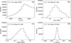 |
Fig. 3 Histograms of (a) Teff, (b) log g, (c) [Fe/H], and (d) Vr of the 861 505 solar-like stars employed in this work. |
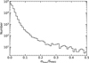 |
Fig. 4 Histogram of |
![Mathematical equation: $\[\sigma_{S_{\mathrm{MWO}}}\]$](/articles/aa/full_html/2024/08/aa48988-23/aa48988-23-eq14.png)
![Mathematical equation: $\[\sigma_{S_{\mathrm{MWO}}}\]$](/articles/aa/full_html/2024/08/aa48988-23/aa48988-23-eq15.png)
3.2 Conversion of SMWO to RHK
In order to connect with a physical quantity, the SMWO can be described by the stellar surface fluxes as
![Mathematical equation: $\[S_{\mathrm{MWO}}=8 \alpha \cdot \frac{\mathcal{F}_{\mathrm{HK}}}{\mathcal{F}_{\mathrm{RV}}},\]$](/articles/aa/full_html/2024/08/aa48988-23/aa48988-23-eq19.png) (5)
(5)
where ![Mathematical equation: $\[\mathcal{F}\]$](/articles/aa/full_html/2024/08/aa48988-23/aa48988-23-eq20.png) HK is the stellar surface flux in the 1.09 Å FWHM H and K bands, and
HK is the stellar surface flux in the 1.09 Å FWHM H and K bands, and ![Mathematical equation: $\[\mathcal{F}\]$](/articles/aa/full_html/2024/08/aa48988-23/aa48988-23-eq21.png) RV represents the stellar surface flux in the 20 Å R and V bands (Vaughan et al. 1978; Middelkoop 1982; Rutten 1984; Hall et al. 2007; Mittag et al. 2013; Marvin et al. 2023). The constant, eight, comes from the aforementioned different exposure times in HKP-2, and α represents the scaling factor in Eq. (2) (Vaughan et al. 1978). The
RV represents the stellar surface flux in the 20 Å R and V bands (Vaughan et al. 1978; Middelkoop 1982; Rutten 1984; Hall et al. 2007; Mittag et al. 2013; Marvin et al. 2023). The constant, eight, comes from the aforementioned different exposure times in HKP-2, and α represents the scaling factor in Eq. (2) (Vaughan et al. 1978). The ![Mathematical equation: $\[\mathcal{F}\]$](/articles/aa/full_html/2024/08/aa48988-23/aa48988-23-eq22.png) RV mainly depends on the stellar atmospheric parameters; thus, it can be derived from empirical spectral library (e.g., Middelkoop 1982; Rutten 1984; Cincunegui et al. 2007; Suárez Mascareño et al. 2015; Astudillo-Defru et al. 2017; Lorenzo-Oliveira et al. 2018) or synthetic spectral library (e.g., Mittag et al. 2013; Pérez Martínez et al. 2014; Marvin et al. 2023). By combining the SMWO with corresponding stellar continuum spectra of the empirical or synthetic spectral library, a new active index RHK can be constructed as follows, which describes the emission of Ca II H and K lines more physically than SMWO (e.g., Linsky et al. 1979; Middelkoop 1982; Rutten 1984; Noyes et al. 1984).
RV mainly depends on the stellar atmospheric parameters; thus, it can be derived from empirical spectral library (e.g., Middelkoop 1982; Rutten 1984; Cincunegui et al. 2007; Suárez Mascareño et al. 2015; Astudillo-Defru et al. 2017; Lorenzo-Oliveira et al. 2018) or synthetic spectral library (e.g., Mittag et al. 2013; Pérez Martínez et al. 2014; Marvin et al. 2023). By combining the SMWO with corresponding stellar continuum spectra of the empirical or synthetic spectral library, a new active index RHK can be constructed as follows, which describes the emission of Ca II H and K lines more physically than SMWO (e.g., Linsky et al. 1979; Middelkoop 1982; Rutten 1984; Noyes et al. 1984).
The stellar surface flux ![Mathematical equation: $\[\mathcal{F}\]$](/articles/aa/full_html/2024/08/aa48988-23/aa48988-23-eq23.png) HK in the 1.09 Å FWHM H and K bands can be normalized by the bolometric flux as
HK in the 1.09 Å FWHM H and K bands can be normalized by the bolometric flux as
![Mathematical equation: $\[R_{\mathrm{HK}}=\frac{\mathcal{F}_{\mathrm{HK}}}{\sigma T_{\mathrm{eff}}^4},\]$](/articles/aa/full_html/2024/08/aa48988-23/aa48988-23-eq24.png) (6)
(6)
where Teff is the stellar effective temperature and σ = 5.67 × 10⁻⁵ erg cm−2 s−1 K−4 is the Stefan-Boltzmann constant. RHK is not related to the continuum flux around the Ca II H and K lines, which is governed by the stellar effective temperature, and thus it can be used to compare stars with different spectral types.
A widely used form of the relationship between SMWO and RHK can be expressed as
![Mathematical equation: $\[R_{\mathrm{HK}}=K \cdot \sigma^{-1} \cdot 10^{-14} \cdot C_{\mathrm{cf}} \cdot S_{\mathrm{MWO}} \text {, }\]$](/articles/aa/full_html/2024/08/aa48988-23/aa48988-23-eq25.png) (7)
(7)
where Ccf is the bolometric factor and 10−14 is an arbitrary factor (Middelkoop 1982; Rutten 1984). The factor K is in units of erg cm−2 s−1, which was introduced by Middelkoop (1982) to convert the relative flux FHK (in arbitrary units),
![Mathematical equation: $\[F_{\mathrm{HK}}=C_{\mathrm{cf}} \cdot T_{\mathrm{eff}}^4 \cdot 10^{-14} \cdot S_{\mathrm{MWO}},\]$](/articles/aa/full_html/2024/08/aa48988-23/aa48988-23-eq26.png) (8)
(8)
to stellar surface flux ![Mathematical equation: $\[\mathcal{F}\]$](/articles/aa/full_html/2024/08/aa48988-23/aa48988-23-eq27.png) HK by
HK by
![Mathematical equation: $\[\mathcal{F}_{\mathrm{HK}}=K \cdot F_{\mathrm{HK}}.\]$](/articles/aa/full_html/2024/08/aa48988-23/aa48988-23-eq28.png) (9)
(9)
The factor Ccf in Eq. (7) was derived by the pioneering studies of Middelkoop (1982) and Rutten (1984) (see, e.g., Noyes et al. 1984; Henry et al. 1996; Wright et al. 2004; Hall et al. 2007; Egeland et al. 2017; Karoff et al. 2019; Sowmya et al. 2021; Gomes da Silva et al. 2021). Middelkoop (1982) first introduced and deduced the Ccf as a function of B − V for main-sequence stars with 0.45 ≤ B − V ≤ 1.5. Subsequently, Rutten (1984) broadened the Ccf to 0.3 ≤ B − V ≤ 1.6 for FGK-type main-sequence stars. To describe the chromospheric activity of an M dwarf, Cincunegui et al. (2007) calibrated Ccf to the 0.45 ≤ B − V ≤ 1.81 range for stars with spectral types ranging from F6 to M5, and Suárez Mascareño et al. (2015) calibrated the Ccf in the range of 0.4 ≲ B − V ≲ 1.9. On the other hand, Astudillo-Defru et al. (2017) derived the Ccf in the range of 0.54 ≤ B − V ≤ 1.90 to include the M dwarf, and they prefer the forms of Ccf described by the color indexes I − K and V − K. Lorenzo-Oliveira et al. (2018) calibrated the Ccf to a function of Teff.
The preceding researches of Ccf are based on empirical method, which can also be obtained from synthetic spectral library. The PHOENIX model atmospheres were utilized by Mittag et al. (2013) to obtain ![Mathematical equation: $\[\mathcal{F}\]$](/articles/aa/full_html/2024/08/aa48988-23/aa48988-23-eq29.png) RV for main-sequence stars, and the relation between
RV for main-sequence stars, and the relation between ![Mathematical equation: $\[\mathcal{F}\]$](/articles/aa/full_html/2024/08/aa48988-23/aa48988-23-eq30.png) RV and B − V is given as
RV and B − V is given as
![Mathematical equation: $\[\log \frac{\mathcal{F}_{\mathrm{RV}}}{19.2}=8.33-1.79(B-V),\]$](/articles/aa/full_html/2024/08/aa48988-23/aa48988-23-eq31.png) (10)
(10)
where 0.44 ≤ B − V ≤ 1.6 and the constant 19.2 is equal to the scaling factor 8α in Eq. (5). ![Mathematical equation: $\[\mathcal{F}\]$](/articles/aa/full_html/2024/08/aa48988-23/aa48988-23-eq32.png) RV is comparable with Ccf, which can be transferred to Ccf through
RV is comparable with Ccf, which can be transferred to Ccf through
![Mathematical equation: $\[C_{\mathrm{cf}}=\frac{\mathcal{F}_{\mathrm{RV}}}{8 \alpha \cdot K \cdot T_{\mathrm{eff}}^4 \cdot 10^{-14}},\]$](/articles/aa/full_html/2024/08/aa48988-23/aa48988-23-eq33.png) (11)
(11)
based on Eqs. (5), (8), and (9). Through matching the PHOENIX spectral library with observed spectra, Pérez Martínez et al. (2014) introduced a quadratic formula of Ccf within 0.44 ≤ B − V ≤ 1.33 for luminosity classes V and IV with log g between 5.0 and 3.5 dex. Marvin et al. (2023) derived the Ccf as a fifth-order function of Teff based on the synthetic spectral library of PHOENIX.
The Ccf in various works described above can generally be expressed with a polynomial:
![Mathematical equation: $\[\log C_{\mathrm{cf}}(X)=\sum_{i=0}^5 C_i X^i,\]$](/articles/aa/full_html/2024/08/aa48988-23/aa48988-23-eq34.png) (12)
(12)
where X represents B − V or Teff, and Ci (i = 0, ..., 5) are the corresponding coefficients presented in Table 1.
The SMWO can be derived from observed spectra, and Ccf can be estimated by stellar color index or Teff as described above. The remaining coefficient in Eq. (7) to be determined is the factor K. Middelkoop (1982) deduced the K = (0.76 ± 0.11) × 106 erg cm−2 s−1 based on the investigation of Linsky et al. (1979); thus, K · σ−1 · 10−14 = 1.34 × 10⁻⁴, which is frequently adopted in the relevant works (e.g., Cincunegui et al. 2007; Pérez Martínez et al. 2014; Suárez Mascareño et al. 2015; Boro Saikia et al. 2018; Gomes da Silva et al. 2021). Rutten (1984) derived K = (1.29 ± 0.19) × 106 erg cm−2 s−1 based on the solar S index SMWO,⊙ = 0.160 (Oranje 1983) and the color index of the Sun (B − V)⊙ = 0.665 (Hardorp 1980). Additionally, Hall et al. (2007) conducted a recalibration of the K value, obtaining a result of (1.07 ± 0.13) × 106 erg cm−2 s−1. They pointed out that the discrepancy between their result and the K value reported by Rutten (1984) is mainly due to the adoption of a different solar B − V value, which they took to be 0.642 (Cayrel de Strobel 1996). K · σ−1 · 10−14 = 1.887 × 10⁻⁴ is gradually adopted in recent works (e.g., Astudillo-Defru et al. 2017; Melbourne et al. 2020; Boudreaux et al. 2022; Marvin et al. 2023).
In this work, the value of RHK derived from the method in the classic literature for the LRS spectra is denoted as RHK,classic, which is calculated by utilizing the Ccf from Rutten (1984) (row 2 in Table 1) and K = 0.76 × 10⁶ erg cm−2 s−1 from Middelkoop (1982). Since the value of B − V is needed for the estimation of RHK,classic, we used the relation between Teff and B − V introduced in Noyes et al. (1984) to transform Teff to B − V when calculating RHK,classic, which is based on the research of Johnson (1966). The transformation is given by
![Mathematical equation: $\[\log ~T_{\mathrm{eff}}=3.908-0.234(B-V),\]$](/articles/aa/full_html/2024/08/aa48988-23/aa48988-23-eq35.png) (13)
(13)
in the 0.4 < B − V < 1.4 range.
Based on Eqs. (5) and (6), we can express RHK by SMWO and ![Mathematical equation: $\[\mathcal{F}\]$](/articles/aa/full_html/2024/08/aa48988-23/aa48988-23-eq36.png) RV as
RV as
![Mathematical equation: $\[R_{\mathrm{HK}}=\frac{S_{\mathrm{MWO}} \cdot \mathcal{F}_{\mathrm{RV}}}{8 \alpha} \cdot \frac{1}{\sigma T_{\mathrm{eff}}^4}.\]$](/articles/aa/full_html/2024/08/aa48988-23/aa48988-23-eq37.png) (14)
(14)
As described above, recent studies have demonstrated that the PHOENIX model is a useful tool for deriving the stellar surface flux ![Mathematical equation: $\[\mathcal{F}\]$](/articles/aa/full_html/2024/08/aa48988-23/aa48988-23-eq38.png) RV. In this work, besides RHK,classic we also utilized the spectral library of PHOENIX to estimate
RV. In this work, besides RHK,classic we also utilized the spectral library of PHOENIX to estimate ![Mathematical equation: $\[\mathcal{F}\]$](/articles/aa/full_html/2024/08/aa48988-23/aa48988-23-eq39.png) RV, and then derive RHK through Eq. (14), denoted as RHK,PHOENIX. Because the detailed stellar atmospheric parameters (Teff, log g and [Fe/H]) are available for LAMOST (see Sect. 2), and the
RV, and then derive RHK through Eq. (14), denoted as RHK,PHOENIX. Because the detailed stellar atmospheric parameters (Teff, log g and [Fe/H]) are available for LAMOST (see Sect. 2), and the ![Mathematical equation: $\[\mathcal{F}\]$](/articles/aa/full_html/2024/08/aa48988-23/aa48988-23-eq40.png) RV values estimated from the PHOENIX synthetic spectra library are related to these stellar parameters, we evaluated the values of RHK,PHOENIX taking these parameters into account.
RV values estimated from the PHOENIX synthetic spectra library are related to these stellar parameters, we evaluated the values of RHK,PHOENIX taking these parameters into account.
Husser et al. (2013) published a high-resolution synthetic spectral library3 based on version 16 of the PHOENIX model atmospheres. The stellar atmospheric parameter space of their library covers 2300 ≤ Teff ≤ 12000 K, 0.0 ≤ log g ≤ 6.0 dex, and −4.0 ≤ [Fe/H] ≤ 1.0 dex. In Lançon et al. (2021), a comparison between the PHOENIX synthetic spectra library and empirical spectra was conducted, and their results show that the spectra of Husser et al. (2013) exhibit good consistency with the empirical spectra in the effective temperature range down to about 4000 K. Considering the stellar parameter space of the LAMOST LRS spectra of solar-like stars used in this work as described in Sect. 2, we utilized the spectra in Husser et al. (2013) within the range of 4800 ≤ Teff ≤ 6300 K, 3.5 ≤ log g ≤ 5.0 dex, and −1.0 ≤ [Fe/H] ≤ 1.0 dex. A total of 320 high-resolution synthetic spectra in this parameter range were collected to calculate the value of ![Mathematical equation: $\[\mathcal{F}\]$](/articles/aa/full_html/2024/08/aa48988-23/aa48988-23-eq41.png) RV. We fit log
RV. We fit log ![Mathematical equation: $\[\mathcal{F}\]$](/articles/aa/full_html/2024/08/aa48988-23/aa48988-23-eq42.png) RV by a ternary quadratic polynomial:
RV by a ternary quadratic polynomial:
![Mathematical equation: $\[\begin{aligned}\log \mathcal{F}_{\mathrm{RV}}= & -138.7639+70.3122 X+0.3893 Y-2.3216 Z, \\& -0.0806 X \cdot Y-0.5840 X \cdot Z+0.0124 Y \cdot Z \\& -8.2986 X^2-0.01242 Y^2-0.0351 Z^2,\end{aligned}\]$](/articles/aa/full_html/2024/08/aa48988-23/aa48988-23-eq43.png) (15)
(15)
where X, Y, and Z represent log Teff, log g, and [Fe/H], respectively. The fitting coefficients are calculated by the nonlinear least-squares method through the python module curve_fit of scipy.optimize (Virtanen et al. 2020). In Fig. 5, we present the relationships between ![Mathematical equation: $\[\mathcal{F}\]$](/articles/aa/full_html/2024/08/aa48988-23/aa48988-23-eq44.png) RV and B − V (or Teff) adopted in different works. The
RV and B − V (or Teff) adopted in different works. The ![Mathematical equation: $\[\mathcal{F}\]$](/articles/aa/full_html/2024/08/aa48988-23/aa48988-23-eq45.png) RV values of the PHOENIX spectra used for deriving Eq. (15) are shown by the gray circles. The solid black line in Fig. 5 is derived from Eq. (15) with log g = 4.44 dex and [Fe/H] = 0.0 dex (solar parameters). It can be seen from Fig. 5 that the results of Hall et al. (2007) (K = 1.07 × 10⁶ erg cm−2 s−1 and Ccf taken from Middelkoop 1982) using empirical spectra library are relatively close to those calculated from the PHOENIX synthetic spectral library.
RV values of the PHOENIX spectra used for deriving Eq. (15) are shown by the gray circles. The solid black line in Fig. 5 is derived from Eq. (15) with log g = 4.44 dex and [Fe/H] = 0.0 dex (solar parameters). It can be seen from Fig. 5 that the results of Hall et al. (2007) (K = 1.07 × 10⁶ erg cm−2 s−1 and Ccf taken from Middelkoop 1982) using empirical spectra library are relatively close to those calculated from the PHOENIX synthetic spectral library.
The ![Mathematical equation: $\[\mathcal{F}\]$](/articles/aa/full_html/2024/08/aa48988-23/aa48988-23-eq52.png) HK,PHOENIX value of the Sun is estimated to be (2.423 ± 0.007) × 106 erg cm−2 s−1, which is calculated by Eqs. (5) and (15) with Teff = 5777 K, log g = 4.44 dex, [Fe/H] = 0.0 dex, and SMWO,⊙ = 0.1694 ± 0.0005. The selected values of solar Teff and log g follow Ramírez et al. (2012). The SMWO,⊙ is the mean value of the solar S index that was obtained from the MWO HKP-2 measurements by Egeland et al. (2017). The solar
HK,PHOENIX value of the Sun is estimated to be (2.423 ± 0.007) × 106 erg cm−2 s−1, which is calculated by Eqs. (5) and (15) with Teff = 5777 K, log g = 4.44 dex, [Fe/H] = 0.0 dex, and SMWO,⊙ = 0.1694 ± 0.0005. The selected values of solar Teff and log g follow Ramírez et al. (2012). The SMWO,⊙ is the mean value of the solar S index that was obtained from the MWO HKP-2 measurements by Egeland et al. (2017). The solar ![Mathematical equation: $\[\mathcal{F}\]$](/articles/aa/full_html/2024/08/aa48988-23/aa48988-23-eq53.png) HK values estimated by Oranje (1983), Hall et al. (2007), and Mittag et al. (2013) are (2.17 ± 0.32) × 106, (2.12 ± 0.25) × 106, and (2.47 ± 0.10) × 106 erg cm−2 s−1, respectively. Our evaluation of
HK values estimated by Oranje (1983), Hall et al. (2007), and Mittag et al. (2013) are (2.17 ± 0.32) × 106, (2.12 ± 0.25) × 106, and (2.47 ± 0.10) × 106 erg cm−2 s−1, respectively. Our evaluation of ![Mathematical equation: $\[\mathcal{F}\]$](/articles/aa/full_html/2024/08/aa48988-23/aa48988-23-eq54.png) HK,⊙ value is consistent with those values estimated in previous investigations with a slight deviation. The deviation may originate from the different spectral fluxes in the PHOENIX model, the different choices of solar atmospheric parameters, and the different value of SMWO,⊙. As a result, the values of RHK,PHOENIX are relatively high compared to RHK,classic, with a boost factor of β = 1.6. Figure 6 displays a comparison between the values of log
HK,⊙ value is consistent with those values estimated in previous investigations with a slight deviation. The deviation may originate from the different spectral fluxes in the PHOENIX model, the different choices of solar atmospheric parameters, and the different value of SMWO,⊙. As a result, the values of RHK,PHOENIX are relatively high compared to RHK,classic, with a boost factor of β = 1.6. Figure 6 displays a comparison between the values of log ![Mathematical equation: $\[\left(\frac{1}{B} R_{\mathrm{HK}, \mathrm{PHOENIX}}\right)\]$](/articles/aa/full_html/2024/08/aa48988-23/aa48988-23-eq55.png) and log RHK,classic for the LAMOST LRS spectra of solar-like stars used in this work. The correlation between them can be fit by a linear formula:
and log RHK,classic for the LAMOST LRS spectra of solar-like stars used in this work. The correlation between them can be fit by a linear formula:
![Mathematical equation: $\[\log R_{\mathrm{HK}, \mathrm{classic}}=1.027 \log \left(\frac{1}{\beta} R_{\mathrm{HK}, \mathrm{PHOENIX}}\right)+0.135 \text {. }\]$](/articles/aa/full_html/2024/08/aa48988-23/aa48988-23-eq56.png) (16)
(16)
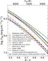 |
Fig. 5 Relations between log |
![Mathematical equation: $\[\mathcal{F}\]$](/articles/aa/full_html/2024/08/aa48988-23/aa48988-23-eq46.png)
![Mathematical equation: $\[\mathcal{F}\]$](/articles/aa/full_html/2024/08/aa48988-23/aa48988-23-eq47.png)
![Mathematical equation: $\[\mathcal{F}\]$](/articles/aa/full_html/2024/08/aa48988-23/aa48988-23-eq48.png)
![Mathematical equation: $\[\mathcal{F}\]$](/articles/aa/full_html/2024/08/aa48988-23/aa48988-23-eq49.png)
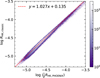 |
Fig. 6 Scatter diagram between log |
![Mathematical equation: $\[\left(\frac{1}{B} R_{\mathrm{HK}, \mathrm{PHOENIX}}\right)\]$](/articles/aa/full_html/2024/08/aa48988-23/aa48988-23-eq50.png)
![Mathematical equation: $\[\left(\frac{1}{B} R_{\mathrm{HK}, \mathrm{PHOENIX}}\right)\]$](/articles/aa/full_html/2024/08/aa48988-23/aa48988-23-eq51.png)
3.3 Derivation of the bolometric- and photospheric-calibrated chromospheric activity index R′HK
The emission flux of Ca II H and K lines is known to comprise the fluxes of the stellar photosphere and chromosphere (Hartmann et al. 1984; Noyes et al. 1984). To acquire a purer chromospheric activity index, we need to subtract the photospheric contribution from RHK. The photospheric and bolometric calibrated chromospheric activity index R′HK (Hartmann et al. 1984; Noyes et al. 1984) is defined as
![Mathematical equation: $\[R_{\mathrm{HK}}^{\prime}=R_{\mathrm{HK}}-R_{\text {phot}},\]$](/articles/aa/full_html/2024/08/aa48988-23/aa48988-23-eq57.png) (17)
(17)
for which RHK is described and derived in Sect. 3.2 and Rphot represents the photospheric contribution that is the ratio between the photospheric flux and the bolometric flux:
![Mathematical equation: $\[R_{\mathrm{phot}}=\frac{\mathcal{F}_{\text {phot }}}{\sigma T_{\mathrm{eff}}^4}.\]$](/articles/aa/full_html/2024/08/aa48988-23/aa48988-23-eq58.png) (18)
(18)
Rphot can be derived from an empirical spectral library (e.g., Hartmann et al. 1984; Noyes et al. 1984; Suárez Mascareño et al. 2015; Lorenzo-Oliveira et al. 2018) or synthetic spectral library (e.g., Mittag et al. 2013; Astudillo-Defru et al. 2017; Marvin et al. 2023). The values of log Rphot in the literature that can be expressed by the polynomial form
![Mathematical equation: $\[\log R_{\text {phot }}=\sum_{i=0}^5 P_i X^i\]$](/articles/aa/full_html/2024/08/aa48988-23/aa48988-23-eq59.png) (19)
(19)
are presented in Table 2. In Eq. (19), X represents B − V or Teff and the Pi (i = 1,...,5) are the coefficients of the polynomial which are given in Table 2.
Noyes et al. (1984) distilled the result of Hartmann et al. (1984) and expressed the relation between log Rphot and B − V via a cubic polynomial,
![Mathematical equation: $\[\log R_{\text {phot }}=-4.898+1.918(B-V)^2-2.893(B-V)^3 \text {, }\]$](/articles/aa/full_html/2024/08/aa48988-23/aa48988-23-eq60.png) (20)
(20)
for the main-sequence stars with B − V > 0.44 (see first row of Table 2). They noted that Rphot becomes negligible for the case of B − V ≳ 1.0. This expression of Rphot in Eq. (20) was widely adopted to derive R′HK in the majority of research (e.g., Henry et al. 1996; Wright et al. 2004; Gray et al. 2006; Gomes da Silva et al. 2021), while a simpler linear form of log Rphot is also available (used in Cincunegui et al. 2007). By cross-matching 72 stars with Noyes et al. (1984), Lorenzo-Oliveira et al. (2018) fit the log Rphot into a formula of Tef,f
![Mathematical equation: $\[\log R_{\text {phot }}=-4.78845-\frac{3.70700}{1+\left(T_{\text {eff }} / 4598.92\right)^{17.527}},\]$](/articles/aa/full_html/2024/08/aa48988-23/aa48988-23-eq61.png) (21)
(21)
for stars in the range of 4350 ≤ Teff ≤ 6500 K. Based on the inactive stars observed by HARPS spectra, Suárez Mascareño et al. (2015) empirically fit the Rphot for the main-sequence star in the 0.4 ≲ B − V ≲ 1.9 range, which is expressed by an exponential function:
![Mathematical equation: $\[R_{\text {phot }}=1.48 \times 10^{-4} \cdot e^{-4.3658(B-V)} \text {. }\]$](/articles/aa/full_html/2024/08/aa48988-23/aa48988-23-eq62.png) (22)
(22)
Mittag et al. (2013) adopted the synthetic spectra of PHOENIX to deduce the photospheric flux ![Mathematical equation: $\[\mathcal{F}\]$](/articles/aa/full_html/2024/08/aa48988-23/aa48988-23-eq63.png) phot, which is expressed by a linear equation for main-sequence star in the range of 0.44 ≤ B − V ≤ 1.28, such as
phot, which is expressed by a linear equation for main-sequence star in the range of 0.44 ≤ B − V ≤ 1.28, such as
![Mathematical equation: $\[\log \mathcal{F}_{\text {phot }}=7.49-2.06(B-V) \text {, }\]$](/articles/aa/full_html/2024/08/aa48988-23/aa48988-23-eq64.png) (23)
(23)
which can be converted to Rphot by Eq. (18).
Astudillo-Defru et al. (2017) derived the Rphot in the range of 0.54 ≤ B − V ≤ 1.90 based on the BT-Settl model (Allard 2014). Moreover, Marvin et al. (2023) employed the PHOENIX model to deduce a fifth-order equation that expresses the log Rphot as a function of Teff. For the same stellar B − V or Teff value, the values of Rphot deduced by synthetic spectra in Mittag et al. (2013), Astudillo-Defru et al. (2017), and Marvin et al. (2023) are generally higher than the empirical calibration of Noyes et al. (1984). Marvin et al. (2023) thus introduced an offset 0.4612 to scale their result to Noyes et al. (1984).
Same as RHK described in Sect. 3.2, we employed two kinds of estimations of R′HK, denoted as R′HK,classic and R′HK,PHOENIX, respectively. R′HK,classic is calculated using RHK,classic and the photospheric contribution derived from Eq. (20) with B − V estimated from Eq. (13), while R′HK,PHOENIX is computed based on RHK,PHOENIX and the photospheric contribution Rphot,PHOENIX estimated as follows.
Because the values of RHK,PHOENIX are approximately β times larger than the values of RHK,classic, we introduced a β-coefflcient to scale Rphot,classic to Rphot,PHOENIX and the corresponding log Rphot,PHOENIX can be expressed by
![Mathematical equation: $\[\begin{aligned}\log R_{\text {phot,PHOENIX }} & =\log \left(\beta \cdot R_{\text {phot,classic }}\right) \\& =-4.694+1.918(B-V)^2-2.893(B-V)^3,\end{aligned}\]$](/articles/aa/full_html/2024/08/aa48988-23/aa48988-23-eq65.png) (24)
(24)
for B − V > 0.44. In Fig. 7, we present the relations between log Rphot and B − V (or Teff) adopted in different works. As discussed above, the Rphot,PHOENIX is scaled from the results of Noyes et al. (1984) using a scale factor β related to the method based on the PHOENIX model. Hence, the solid red curve in Fig. 7 differs from those obtained in Mittag et al. (2013) and Marvin et al. (2023).
Since the detailed stellar atmospheric parameters (Teff, log g and [Fe/H]) are available for LAMOST, we estimated the B − V in Eq. (24) by considering not only Teff, but also the stellar atmospheric parameters log g and [Fe/H]. Based on the InfraRed Flux Method, Casagrande et al. (2010) found that there is very little dependence of B − V on log g and provided a relation between Teff, B − V, and [Fe/H], with B − V and [Fe/H] in the range of 0.18 ≤ B − V ≤ 1.29 and −5.0 ≤ [Fe/H] ≤ 0.4 dex. We examine the extendability of the [Fe/H] upper boundary and still employ the relation to obtain the B − V for the small amount of spectra with [Fe/H] slightly exceeding 0.4 dex. After obtaining B − V from Teff and [Fe/H], we then estimate the photospheric contribution Rphot,PHOENIX based on Eq. (24). Because both the RHK,PHOENIX and Rphot,PHOENIX are about β times higher than the corresponding classic indexes, to be consistent with classic studies, we calculated the R′HK,PHOENIX by
![Mathematical equation: $\[R_{\mathrm{HK}, \mathrm{PHOENIX}}^{\prime}=\frac{1}{\beta}\left(R_{\mathrm{HK}, \mathrm{PHOENIX}}-R_{\text {phot,PHOENIX }}\right).\]$](/articles/aa/full_html/2024/08/aa48988-23/aa48988-23-eq66.png) (25)
(25)
In Fig. 8, we present a comparison between the values of the two indexes log R′HK,PHOENIX and log R′HK,classic for the LAMOST LRS spectra of solar-like stars studied in this work. As shown in Fig. 8, there exists a linear correlation between these two quantities; the fitting formula is
![Mathematical equation: $\[\log R_{\mathrm{HK}, \text { classic }}^{\prime}=0.999 \log R_{\mathrm{HK}, \mathrm{PHOENIX}}^{\prime}+0.009 \text {. }\]$](/articles/aa/full_html/2024/08/aa48988-23/aa48988-23-eq67.png) (26)
(26)
Egeland et al. (2017) estimated the average value of log R′HK,⊙ as −4.9427 ± 0.0072 based on the SMWO,⊙ in the 15–24 solar cycle and (B − V)⊙ = 0.653 ± 0.003. Taking Teff = 5777 K, log g = 4.44 dex, [Fe/H] = 0.0 dex, and the same solar B − V, we can obtain the log R′HK,PHOENIX = −4.9599 ± 0.0051 for the Sun.
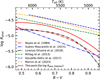 |
Fig. 7 Relations between log Rphot and B − V (or Teff) adopted in different researches. The formulas derived from empirical and synthetic spectral libraries in the literature are indicated by dashed-dotted and dashed lines, respectively. The formula of log Rphot,PHOENIX adopted in this work is indicated by the solid red line. |
3.4 Estimation of the uncertainty of chromospheric activity indexes
We estimated the uncertainties of log RHK,classic, log R′HK,classic, log RHK,PHOENIX, and log R′HK,PHOENIX with the Monte Carlo error propagation. Because the log RHK,PHOENIX values are calculated by Eq. (14), the uncertainties of log RHK,PHOENIX are yielded from the uncertainties of SMWO and ![Mathematical equation: $\[\mathcal{F}\]$](/articles/aa/full_html/2024/08/aa48988-23/aa48988-23-eq68.png) RV. The uncertainties of log RHK,classic predominantly arise from the uncertainties of SMWO and Ccf as presented in Eq. (7). As illustrated in Paper I, we estimated the uncertainties of SMWO by considering the impact of the uncertainties of the spectral flux, the discretization in spectral data, and the uncertainty of radial velocity. The uncertainties of
RV. The uncertainties of log RHK,classic predominantly arise from the uncertainties of SMWO and Ccf as presented in Eq. (7). As illustrated in Paper I, we estimated the uncertainties of SMWO by considering the impact of the uncertainties of the spectral flux, the discretization in spectral data, and the uncertainty of radial velocity. The uncertainties of ![Mathematical equation: $\[\mathcal{F}\]$](/articles/aa/full_html/2024/08/aa48988-23/aa48988-23-eq69.png) RV are affected by the uncertainties of stellar atmospheric parameters Teff, log g, and [Fe/H] due to Eq. (15). Since we calculate the value of Ccf through the B − V value derived from Eq. (13), the uncertainties of Ccf are influenced by the uncertainties of B − V that are propagated from the uncertainties of Teff.
RV are affected by the uncertainties of stellar atmospheric parameters Teff, log g, and [Fe/H] due to Eq. (15). Since we calculate the value of Ccf through the B − V value derived from Eq. (13), the uncertainties of Ccf are influenced by the uncertainties of B − V that are propagated from the uncertainties of Teff.
Figure 9a illustrates the histograms of the uncertainties of log SMWO, log Ccf, log RHK,classic, log Rphot,classic and log R′HK,classic, while Fig. 9b shows the uncertainties for log SMWO, log ![Mathematical equation: $\[\mathcal{F}\]$](/articles/aa/full_html/2024/08/aa48988-23/aa48988-23-eq70.png) RV, log RHK,PHOENIX, log Rphot,PHOENIX and log R′HK,PHOENIX shown in Fig. 9, the uncertainties of log RHK,PHOENIX and log RHK,classic are both primarily governed by the uncertainties of SMWO. The uncertainties of log SMWO; log RHK,classic, log R′HK,classic log RHK,PHOENIX, and log R′HK,PHOENIX are distributed around 0.030, 0.030, 0.065, 0.030, and 0.065, respectively.
RV, log RHK,PHOENIX, log Rphot,PHOENIX and log R′HK,PHOENIX shown in Fig. 9, the uncertainties of log RHK,PHOENIX and log RHK,classic are both primarily governed by the uncertainties of SMWO. The uncertainties of log SMWO; log RHK,classic, log R′HK,classic log RHK,PHOENIX, and log R′HK,PHOENIX are distributed around 0.030, 0.030, 0.065, 0.030, and 0.065, respectively.
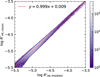 |
Fig. 8 Scatter diagram between log R′HK,PHOENIX and log R′HK,classic for LAMOST LRS spectra of solar-like stars studied in this work. The color scale represents the density of data points. The dashed line is the linear fit between log R′HK,PHOENIX and log R′HK,classic. |
4 Results and discussion
4.1 Stellar chromospheric activity database
In Sect. 3, we investigate the stellar chromospheric activity via two method types. The chromospheric activity parameters derived from the method in the classic literature are denoted as classic, while those derived from the method based on the PHOENIX model are denoted as PHOENIX. We provide the database4 of chromospheric activity parameters for 1 122 495 LAMOST LRS spectra of solar-like stars, which is compiled in a CSV format file: CaIIHK_Activity_Indexes_ LAMOST_DR8_LRS.csv. The database mainly includes the chromospheric activity parameters Stri, SMMO, RHK,classic, R′HK,classic, RHK,PHOENIX, and R′HK,PHOENIX, as well as their uncertainties. The columns in the catalog of the database are presented in Table 3.
The log R′HK,classic and log R′HK,PHOENIX values of 743 and 821 spectra, respectively, are not available (recorded as “−9999” in the database). One of the reasons is that the value of stellar parameters exceeds the valid range of the empirical formula of Rphot (0 and 13 spectra for classic and PHOENIX, respectively). The other reason is that the estimated value of photospheric contribution is larger than the value of RHK for very few spectra (743 and 808 spectra for classic and PHOENIX, respectively). This situation occurs either because the photospheric contributions are determined empirically, leading to overestimations for some stars; or because there are uncertainties in the evaluation of RHK. These spectra are not involved in the subsequent discussion. In Sects. 3.2 and 3.3, we detail comparisons between log RHK,classic and log RHK,PHOENIX and between log R′HK,classic and log R′HK,PHOENIX. The results indicate that log RHK,PHOENIX and log R′HK,PHOENIX are approximately linearly correlated with log RHK,classic and log RHK,classic, respectively (see Figs. 6 and 8). In the next subsection, we discuss the distribution of chromospheric activity primarily based on RHK,PHOENIX and R′HK,PHOENIX.
4.2 Distribution of chromospheric activity index
Among the 1 122 495 LAMOST LRS spectra of solar-like stars, there are 861 505 stars with a gaia_source_id available in LAMOST LRS AFGK Catalog. In this section, we investigate the distribution of the chromospheric activity index based on these stars. If a star is recorded more than once in our dataset, we used the median values of the chromospheric activity parameters from the multiple observed spectra. In Paper I, we calibrated the S index of LAMOST to SMWO, and we also compared the R′HK with the results in the literature, as illustrated in Appendix B. There is an approximate consistency between our R′HK values and those from other instruments for the common targets.
In Fig. 10, we display the distribution of log RHK,PHOENIX with Teff for the 861 505 solar-like stars. The solar value of log RHK,PHOENIX (−4.416 ± 0.001) is displayed in Fig. 10 with a * symbol, which is calculated by Eq. (6) with the solar ![Mathematical equation: $\[\mathcal{F}\]$](/articles/aa/full_html/2024/08/aa48988-23/aa48988-23-eq71.png) ,HK,PHOENIX = (2.423 ± 0.007) × 106 erg cm−2 s−1 given in Sect. 3.2.
,HK,PHOENIX = (2.423 ± 0.007) × 106 erg cm−2 s−1 given in Sect. 3.2.
It is not surprising that the distribution trend of log RHK,PHOENIX shows a clear correlation with Teff. Although the RHK,PHOENIX is the bolometric calibration of the surface flux, the photospheric contribution related to stellar spectral types is still contained. As mentioned in Sect. 3.3, it is necessary to further remove the contribution of photosphere to obtain R′HK,PHOENIX. The histograms of the log R′HK,PHOENIX values are exhibited in Figs. 11a and b in linear-scale and logarithmic-scale vertical axes, respectively. The peak of the distribution is at about −4.90. This peak value is close to the solar log R′HK,PHOENIX = −4.9599 as given in Sect. 3.3.
The Vaughan-Preston gap (VP gap, Vaughan & Preston 1980), known as the bimodal distribution of chromospheric activity, is not observed in Fig. 11. The separation of log R′HK values between active and inactive stars may suggest the existence of different dynamo mechanisms (Vaughan & Preston 1980; Noyes et al. 1984; Henry et al. 1996; Jenkins et al. 2006; Gray et al. 2006; Gomes da Silva et al. 2021). Boro Saikia et al. (2018) investigated a global sample of 4451 cool stars from high-resolution HARPS spectra and concluded that the VP gap is not pronounced. A significant proportion of the stars have intermediate activity levels around log R′HK = −4.75 in Boro Saikia et al. (2018). In contrast, the bimodal distribution of chromospheric activity in Gomes da Silva et al. (2021) is relatively significant, based on 1674 F-, G- and K-type stars from the HARPS sample. Gray et al. (2006) and Hinkel et al. (2017) proposed that the VP gap tends to appear for stars with [Fe/H] greater than −0.2, which is inflexible for stars in this work. The VP gap is also influenced by the rotation rate (e.g., Noyes et al. 1984; Rutten 1987), and the relationship between rotation and stellar chromospheric activity in LAMOST samples will be investigated in the future. Vaughan & Preston (1980) suggested that the VP gap might originate from different dynamo mechanisms or statistical bias. The absence of a VP gap in the distribution of chromospheric activity for our solar-like stars could be attributed to three possible factors: 1) a gradual diminishing of chromospheric activity during the evolution of solar-like stars; 2) the influence of different stellar properties on the bimodal distribution of the chromospheric activity within our samples, which should be explored in more detail in the future; or 3) the loss of some information in the spectral profile due to the limited resolution of LAMOST LRS spectra (Jenkins et al. 2011).
We display the distributions of log R′HK,PHOENIX with Teff, log g, and [Fe/H] in Figs. 12a, b, and c, respectively. To show the trends of log R′HK,PHOENIX with these stellar atmospheric parameters, the log R′HK,PHOENIX values are homogeneously segregated into equal-width bins for 4800 < Teff < 6300 K, 3.9 < log g < 4.8 dex and −1.0 < [Fe/H] < 0.6 dex with steps of 50 K, 0.1 dex, and 0.1 dex, respectively; and the fit median values of the log R′HK,PHOENIX in each bin with Teff, log g, and [Fe/H] are marked by the black dashed lines in Fig. 12. The formulas of these fit trends are expressed by the following quadratic polynomials:
![Mathematical equation: $\[\log R_{\mathrm{HK}, \mathrm{PHOENIX}}^{\prime}=4.367-3.397 \times 10^{-3} T_{\mathrm{eff}}+3.094 \times 10^{-7} T_{\mathrm{eff}}^2,\]$](/articles/aa/full_html/2024/08/aa48988-23/aa48988-23-eq72.png) (27)
(27)
![Mathematical equation: $\[\log R_{\mathrm{HK}, \mathrm{PHOENIX}}^{\prime}=1.595-3.166 \log g+0.384(\log g)^2 \text {, }\]$](/articles/aa/full_html/2024/08/aa48988-23/aa48988-23-eq73.png) (28)
(28)
![Mathematical equation: $\[\log R_{\mathrm{HK}, \mathrm{PHOENIX}}^{\prime}=-4.912-0.065[\mathrm{Fe} / \mathrm{H}]+7.894 \times 10^{-3}[\mathrm{Fe} / \mathrm{H}]^2 \text {. }\]$](/articles/aa/full_html/2024/08/aa48988-23/aa48988-23-eq74.png) (29)
(29)
As shown in Fig. 12, the median values of log R′HK,PHOENIX with Teff exhbit a minimum at about Teff = 5500 K, while the dependence of the median values of log R′HK,PHOENIX on log g and [Fe/H] is relatively weak. It can be seen that the solar log R′HK,PHOENIX value is approximately on the fitting lines of the median log R′HK,PHOENIX values for all three parameters, and the value of solar chromospheric activity index is located at the midpoint of the solar-like star sample. This result, based on our extensive archive, supports the view that the dynamo mechanism of solar-like stars is generally consistent with that of the Sun.
Henry et al. (1996) classified the stellar chromospheric activity in four levels: very active (log R′HK larger than −4.20), active (log R′HK from −4.75 to −4.20), inactive (log R′HK from −5.10 to −4.75), and very inactive (log R′HK less than −5.10). Following this classification, based on the log R′HK,PHOENIX values of 861 505 stars, we can obtain the proportions of very active, active, inactive, and very inactive solar-like stars as 1.03%, 21.68%, 65.27%, and 12.03%, respectively. While for the values of log R′HK,classic, the proportions are 1.07%, 24.53%, 62.98%, and 11.41%, respectively. The proportions of stars in the different stellar chromospheric activity classes are 2.6%, 27.1%, 62.5%, and 7.9% in Henry et al. (1996), and 1.2%, 28.5%, 66.9%, and 3.5% in Gomes da Silva et al. (2021). When using a threshold of log R′HK = −4.75 to classify stars as active and inactive, Henry et al. (1996) and Gomes da Silva et al. (2021) found that 29.7% stars are classified as active. Classifying the solar-like stars studied in this work with log R′HK,PHOENIX = −4.75 and log R′HK,classic = −4.75, we can obtain the proportions of active solar-like stars: 22.71% and 25.60%, respectively. The proportions are relatively consistent with the results of Henry et al. (1996) and Gomes da Silva et al. (2021).
In Fig. 13, we show the distributions of log R′HK,PHOENIX values in the Teff versus log g, Teff versus [Fe/H], and [Fe/H] versus log g parameter spaces. The stellar chromospheric activity levels of very active, active, inactive, and very inactive elements are indicated by different colors. It can be seen from Fig. 13 that the higher the stellar chromospheric activity levels, the narrower the distribution areas in the parameter spaces. Since the LAMOST LRS spectra of solar-like stars with determined stellar atmospheric parameters are sufficient, we further investigated the relations between the proportions of solar-like stars with different chromospheric activity levels (classified by R′HK,PHOENIX) and the stellar atmospheric parameters (Teff, log g, and [Fe/H]). The proportions of very active, active, inactive, and very inactive solar-like stars with different stellar atmospheric parameters are shown in Fig. 14. The proportion values in Fig. 14 were obtained by dividing the Teff, log g, and [Fe/H] into bins with step sizes of 100 K, 0.1 dex, and 0.1 dex, respectively; the central values of each bin are used to represent the corresponding stellar atmospheric parameters.
Figure 14a shows that the proportions of inactive solar-like stars exhibit a relatively stable trend within the Teff range of 4800 to 6000 K. For the very inactive solar-like stars, there is an increasing trend in the proportions as the Teff decreases within the Teff range from 6300 to 5650 K, and the proportions decrease within the Teff range from 5650 to 4800 K. In contrast, the proportions of active solar-like stars exhibit a decreasing trend with decreasing Teff from 6300 to 5650 K, and the decreasing trend of the proportions of active solar-like stars is reversed for a Teff lower than 5650 K. The proportions of very active solar-like stars are almost stable for Teff > 5900 K, while they increase for Teff < 5600 K. The minimum value of the proportions of very active solar-like stars is around Teff = 5700 K. Based on the proportions of active and very active solar-like stars, we conclude that the occurrence rate of high levels of chromospheric activity is lower among the stars with effective temperatures between 5600 and 5900 K.
The relations between log g and the proportions of solar-like stars with different chromospheric activity levels are displayed in Fig. 14b. The proportions of different chromospheric activity levels of solar-like stars appear to be relatively stable in the range of 3.9 < log g < 4.5 dex. When log g > 4.5 dex, the proportions of active solar-like stars exhibits an increasing trend, whereas the spectral ratios of very inactive, inactive, and very active solarlike stars decrease.
Gray et al. (2006) and Hinkel et al. (2017) detected that the distribution of log R′HK varies among stars with different levels of metallicity, and the bimodal distribution (Vaughan & Preston 1980) is observed in dwarf stars with an [Fe/H] greater than −0.2 dex. In the research of Jenkins et al. (2008), the majority of stars with [Fe/H] > 0.1 dex were found to be inactive. In Fig. 11, the bimodal distribution of log R′HK does not exist in our solar-like star sample of LAMOST LRS. However, as shown in Fig. 14c, when [Fe/H] > 0.1 dex, there is a decrease in the proportions of active solar-like stars. This decreasing trend ceases, and the proportions of active solar-like stars become relatively stable when [Fe/H] = 0.3 dex.
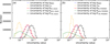 |
Fig. 9 Histograms of uncertainties of parameters derived from (a) the method in the classic literature and (b) the method based on the PHOENIX model. |
Columns in the catalog of the database.
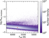 |
Fig. 10 Scatter diagram of log RHK,PHOENIX with Teff for all of solar-like stars investigated in this work. The color scale represents the density of data points. The RHK,PHOENIX value of the Sun is marked with a (*) symbol. |
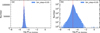 |
Fig. 11 Histograms of log R′HK,PHOENIX values for the solar-like stars investigated in this work through (a) linear-scale and (b) logarithmic-scale vertical axes. The log R′HK,PHOENIX value of the Sun (−4.9599 as given in Sect. 3.3) is indicated by a vertical dashed line. |
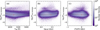 |
Fig. 12 Scatter diagrams of log R′HK,PHOENIX with (a) Teff, (b) log g, and (c) [Fe/H] for the solar-like stars investigated in this work. The position of the solar log R′HK,PHOENIX in these diagrams is denoted by a (*) symbol. The black dashed lines represent the fit median values of log R′HK,PHOENIX The color scale indicates the number density. Some values of log R′HK,PHOENIX outside the displayed range are considered insignificant for the overall distribution and are therefore not shown. |
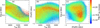 |
Fig. 13 Distributions of log R′HK,PHOENIX values in (a) Teff versus log g, (b) Teff versus [Fe/H], and (c) [Fe/H] versus log g parameter spaces for the solar-like stars investigated in this work. The stellar chromospheric activity levels of very active, active, inactive, and very inactive are indicated by different colors. The values of log R′HK,PHOENIX that fall outside the range of the color bar are represented by the boundary value. The data points with smaller log R′HK,PHOENIX are overlaid by the data points with larger log R′HK,PHOENIX. The positions of the solar log R′HK,PHOENIX are marked in the diagrams with a (*) symbol colored in accordance with the solar activity level. |
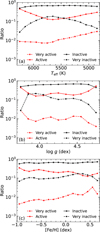 |
Fig. 14 Relations of proportions of very active (red dashed line), active (red line), inactive (black line), and very inactive (black dashed line) solar-like stars with (a) Teff, (b) log g, and (c) [Fe/H]. The proportions values are obtained by dividing the Teff, log g and [Fe/H] into bins with step sizes of 100 K, 0.1 dex, and 0.1 dex, respectively, and the central values of each bin are used to represent the corresponding stellar atmospheric parameters. |
5 Summary and conclusion
In this work, we identify 1 122 495 high-quality LRS spectra of solar-like stars from LAMOST DR8 and provide a database of stellar chromospheric activity parameters based on this spectral sample. The database contains the stellar chromospheric activity parameters Stri, SMWO, RHK, and R′HK, as well as their uncertainties. RHK and R′HK are derived from the method in the classic literature (denoted with classic) and the method based on the PHOENIX model (denoted as PHOENIX). When converting the SMWO to the bolometric calibrated index RHK, the RHK,classic values are estimated based on the bolometric factor Ccf from Rutten (1984) and the K factor from Middelkoop (1982), while the RHK,PHOENIX values are derived from the stellar surface flux ![Mathematical equation: $\[\mathcal{F}\]$](/articles/aa/full_html/2024/08/aa48988-23/aa48988-23-eq75.png) RV. The values of RHK,PHOENIX are approximately β = 1.6 times larger than the values of RHK,classic. For the corresponding photospheric contribution Rphot, the Rphot,classic are deduced based on Noyes et al. (1984), and the Rphot,PHOENIX are scaled by β times from the Rphot,classic. The bolometric- and photosphericcalibrated chromospheric activity index R′HK is consequently derived by eliminating the photospheric contribution from RHK. Our calculations show that log RHK,PHOENIX and log R′HK,PHOENIX are approximately linearly correlated with log RHK,classic and log R′HK,classic, respectively.
RV. The values of RHK,PHOENIX are approximately β = 1.6 times larger than the values of RHK,classic. For the corresponding photospheric contribution Rphot, the Rphot,classic are deduced based on Noyes et al. (1984), and the Rphot,PHOENIX are scaled by β times from the Rphot,classic. The bolometric- and photosphericcalibrated chromospheric activity index R′HK is consequently derived by eliminating the photospheric contribution from RHK. Our calculations show that log RHK,PHOENIX and log R′HK,PHOENIX are approximately linearly correlated with log RHK,classic and log R′HK,classic, respectively.
We explore the overall properties of stellar chromospheric activity based on the 861 505 solar-like stars in the database. The results show that the median values of log R′HK,PHOENIX with Teff have a minimum at about Teff = 5500 K, while the dependence of the median values of log R′HK,PHOENIX on log g and [Fe/H] is relatively weak. The value of solar chromospheric activity index is located at the midpoint of the solar-like star sample. This result from our extensive archive supports the view that the dynamo mechanism of solar-like stars is generally consistent with the Sun. The absence of a VP gap in the distribution of chromospheric activity for our solar-like stars could be attributed to three possible factors: 1) a gradual diminishing of chromospheric activity during the evolution of solar-like stars; 2) the influence of different stellar properties on the bimodal distribution of the chromospheric activity within our samples, which should be explored in more detail in the future; or 3) the loss of some information in the spectral profile due to the limited resolution of LAMOST LRS spectra.
We explored the proportions of solar-like stars with different chromospheric activity levels (very active, active, inactive, and very inactive). Based on the values of log R′HK,PHOENIX, we can obtain the proportions of very active, active, inactive, and very inactive solar-like stars as 1.03%, 21.68%, 65.27%, and 12.03%, respectively. While for the values of log R′HK,classic, the proportions are 1.07%, 24.53%, 62.98%, and 11.41%, respectively. It is observed that the higher the stellar chromospheric activity levels, the narrower the distribution areas in the Teff versus log g, Teff versus [Fe/H], and [Fe/H] versus log g parameters spaces.
We further investigated the relation between the proportions of solar-like stars with different chromospheric activity levels (classified by R′HK,PHOENIX) and the stellar atmospheric parameters (Teff, log g and [Fe/H]). Based on the proportions of active and very active solar-like stars, it is concluded that the occurrence rate of high levels of chromospheric activity is lower among the stars with effective temperatures between 5600 and 5900 K. It is found that when log g > 4.5 dex, the proportions of active solar-like stars exhibit an increasing trend, whereas the proportions of very inactive, inactive, and very active solar-like stars decrease. We discovered that there is a decrease in the proportions of active solar-like stars when [Fe/H] > 0.1 dex. This decreasing trend ceases and the proportions of active solar-like stars become relatively stable when [Fe/H] = 0.3 dex.
The chromospheric activity database of the LAMOST LRS spectra of solar-like stars provided in this work includes the most commonly used chromospheric activity parameters such as SMWO, RHK, and R′HK. The relationship between chromospheric activity and other stellar magnetic manifestation (such as stellar rotation period and age) can be further investigated. Additionally, the database can be used to investigate the relationship between stellar and solar activity for a better understanding of the stellar-solar connection. The database may also contribute to the discovery of new solar-type stars accommodating potentially habitable exoplanetary systems.
Acknowledgements
This work is supported by the National Key R&D Program of China (2019YFA0405000) and the National Natural Science Foundation of China (12073001 and 11973059). W.Z. and J.Z. thank the support of the Anhui Project (Z010118169). H.H. acknowledges the CAS Strategic Pioneer Program on Space Science (XDA15052200) and the B-type Strategic Priority Program of the Chinese Academy of Sciences (XDB41000000). Guoshoujing Telescope (the Large Sky Area Multi-Object Fiber Spectroscopic Telescope, LAMOST) is a National Major Scientific Project built by the Chinese Academy of Sciences. Funding for the project has been provided by the National Development and Reform Commission. LAMOST is operated and managed by the National Astronomical Observatories, Chinese Academy of Sciences.
Appendix A Accuracy of stellar parameters
We identified 3806 common stars in Amard et al. (2020) and compared their effective temperature values with those in our database, as shown in Fig. A.1. For a Teff in the range of 4800 to 6300 K, the Teff values provided by LASP are approximately consistent with the results in Amard et al. (2020); generally, ΔTeff is less than 120 K. The Teff,A2020 values are obtained from various observation instruments and are taken from the survey with the highest spectral resolution when the same sources were observed in multiple surveys (Amard et al. 2020). Differences in observation instruments and estimation methods would contribute to the discrepancies between Teff,LASP and Teff,A2020. Although there are some differences between Teff,LASP and Teff,A2020, the corresponding log R′HK,PHOENIX values estimated based on Teff,LASP and Teff,A2020 exhibit approximate consistency, as shown in Figure A.2, where the Δ log R′HK,PHOENIX values are generally less than 0.05.
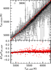 |
Fig. A.1 Distribution of Teff,LASP values and Teff,A2020 values for 3806 common stars, where Teff,A2020 denotes the effective temperature in Amard et al. (2020). The dashed red line represents the case where Teff,LASP equals Teff,A2020. Error bars are indicated for data points that have specified uncertainty values. The lower panel displays the distribution of ΔTeff/Teff,LASP against Teff,LASP, where ΔTeff = Teff,LASP − Teff,A2020. |
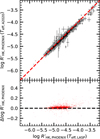 |
Fig. A.2 Scatter plot of log R′HK,PHOENIX (Teff,LASP) versus log R′HK,PHOENIX (Teff,A2020) for stars in Figure A.1. Error bars are displayed for data points with known uncertainty values. The dashed red line represents the ratio of |
![Mathematical equation: $\[\frac{\log R_{\mathrm{HK}, \mathrm{PHOENIX}}^{\prime}\left(T_{\mathrm{eff}, \mathrm{LASP}}\right)}{\left.\log R_{\mathrm{HK}, \mathrm{PHOENIX}}^{\prime} T_{\mathrm{eff}, \mathrm{A} 2020}\right)}=1.\]$](/articles/aa/full_html/2024/08/aa48988-23/aa48988-23-eq76.png)
Appendix B Calibration of chromospheric activity index
We cross-matched the Gaia DR3 source identifier in this paper with stars in Wright et al. (2004), Isaacson & Fischer (2010), Boro Saikia et al. (2018), and Gomes da Silva et al. (2021), and we discovered 23 common stars (16 stars in Wright et al. 2004 and Isaacson & Fischer 2010 are also studied in Boro Saikia et al. 2018). Figure B.1 shows the distribution between log R′HK,PHOENIX and log R′HK,paper. As can be seen in Figure B.1, our results show an approximate agreement with values from other instruments. The values used in Figure B.1 are recorded in Table B.1.
Common stars for comparing log R′HK,PHOENIX with log R′HK,paper in Figure B.1.
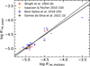 |
Fig. B.1 Distribution of log R′HK,PHOENIX Versus log R′HK,paper. The dashed line represents the case where the log R′HK,PHOENIX is equal to log R′HK,paper, and the solid line is the linear fit between log R′HK,PHOENIX and log R′HK,paper. Data points with quantified uncertainties are represented with error bars. |
Appendix C Distribution of chromospheric activity index with multi-observation
The histogram of σlog R′HK,PHOENIX / log R′HK,PHOENIX for stars with more than one observation is shown in Figure C.1, where the σ log R′HK,PHOENIX represents the standard deviation of log R′HK,PHOENIX. The stars with σ log R′HK,PHOENIX/log R′HK,PHOENIX < 0.2 account for 95.5%of the stars with more than one observation. Additionally, Figure C.2 displays the distributions of log R′HK,PHOENIX with Teff (a), log g (b), and [Fe/H] (c) for solar-like stars with more than one observation and σ log R′HK,PHOENIX / log R′HK,PHOENIX < 0.2. The envelopes in Figure C.2 are similar to those in Figure 12. The distributions of log R′HK,PHOENIX values in (a) Teff versus log g, (b) Teff versus [Fe/H], and (c) [Fe/H] versus log g parameter spaces for solar-like stars with more than one observation and σ log R′HK,PHOENIX / log R′HK,PHOENIX < 0.2 are shown in Figure 13.
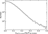 |
Fig. C.1 Histogram of σ log R′HK,PHOENIX / log R′HK,PHOENIX for solar-like stars with more than one observation, where the σ log R′HK,PHOENIX represents the standard deviation of log R′HK,PHOENIX. |
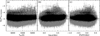 |
Fig. C.2 Distributions of log R′HK,PHOENIX with (a) Teff, (b) log g, and (c) [Fe/H] for solar-like stars with more than one observation and σ log R′HK,PHOENIX / log R′HK,PHOENIX < 0.2. Error bars represent the standard deviation of log R′HK,PHOENIX. |
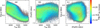 |
Fig. C.3 Distributions of log R′HK,PHOENIX values in (a) Teff versus log g, (b) Teff versus [Fe/H], and (c) [Fe/H] versus log g parameter spaces for solar-like stars with more than one observation and σ log R′HK,PHOENIX / log R′HK,PHOENIX < 0.2. The form of this image is similar to that in Figure 13, where the error bars belong to the bottom end of the data point. |
References
- Ahumada, R., Allende Prieto, C., Almeida, A., et al. 2020, ApJS, 249, 3 [NASA ADS] [CrossRef] [Google Scholar]
- Allard, F. 2014, in Exploring the Formation and Evolution of Planetary Systems, 299, eds. M. Booth, B. C. Matthews, & J. R. Graham, 271 [Google Scholar]
- Allard, F., & Hauschildt, P. H. 1995, ApJ, 445, 433 [NASA ADS] [CrossRef] [Google Scholar]
- Amard, L., Roquette, J., & Matt, S. P. 2020, MNRAS, 499, 3481 [NASA ADS] [CrossRef] [Google Scholar]
- Astudillo-Defru, N., Delfosse, X., Bonfils, X., et al. 2017, A&A, 600, A13 [NASA ADS] [CrossRef] [EDP Sciences] [Google Scholar]
- Bai, Z.-R., Zhang, H.-T., Yuan, H.-L., et al. 2021, Res. Astron. Astrophys., 21, 249 [CrossRef] [Google Scholar]
- Baliunas, S. L., Donahue, R. A., Soon, W. H., et al. 1995, ApJ, 438, 269 [Google Scholar]
- Booth, R. S., Poppenhaeger, K., Watson, C. A., et al. 2020, MNRAS, 491, 455 [NASA ADS] [CrossRef] [Google Scholar]
- Boro Saikia, S., Marvin, C. J., Jeffers, S. V., et al. 2018, A&A, 616, A108 [NASA ADS] [CrossRef] [EDP Sciences] [Google Scholar]
- Boudreaux, T. M., Newton, E. R., Mondrik, N., Charbonneau, D., & Irwin, J. 2022, ApJ, 929, 80 [NASA ADS] [CrossRef] [Google Scholar]
- Brown, E. L., Jeffers, S. V., Marsden, S. C., et al. 2022, MNRAS, 514, 4300 [CrossRef] [Google Scholar]
- Casagrande, L., Ramírez, I., Meléndez, J., Bessell, M., & Asplund, M. 2010, A&A, 512, A54 [NASA ADS] [CrossRef] [EDP Sciences] [Google Scholar]
- Cayrel de Strobel, G. 1996, A&A Rev., 7, 243 [CrossRef] [Google Scholar]
- Ciddor, P. E. 1996, Appl. Opt., 35, 1566 [Google Scholar]
- Cincunegui, C., Díaz, R. F., & Mauas, P. J. D. 2007, A&A, 469, 309 [NASA ADS] [CrossRef] [EDP Sciences] [Google Scholar]
- Cui, X.-Q., Zhao, Y.-H., Chu, Y.-Q., et al. 2012, Res. Astron. Astrophys., 12, 1197 [Google Scholar]
- de Grijs, R., & Kamath, D. 2021, Universe, 7, 440 [NASA ADS] [CrossRef] [Google Scholar]
- Duncan, D. K., Vaughan, A. H., Wilson, O. C., et al. 1991, ApJS, 76, 383 [Google Scholar]
- Egeland, R., Soon, W., Baliunas, S., et al. 2017, ApJ, 835, 25 [NASA ADS] [CrossRef] [Google Scholar]
- Gaia Collaboration (Vallenari, A., et al.) 2023, A&A, 674, A1 [NASA ADS] [CrossRef] [EDP Sciences] [Google Scholar]
- Gomes da Silva, J., Santos, N. C., Adibekyan, V., et al. 2021, A&A, 646, A77 [NASA ADS] [CrossRef] [EDP Sciences] [Google Scholar]
- Gray, R. O., Corbally, C. J., Garrison, R. F., McFadden, M. T., & Robinson, P. E. 2003, AJ, 126, 2048 [Google Scholar]
- Gray, R. O., Corbally, C. J., Garrison, R. F., et al. 2006, AJ, 132, 161 [Google Scholar]
- Gustafsson, B., Edvardsson, B., Eriksson, K., et al. 2008, A&A, 486, 951 [NASA ADS] [CrossRef] [EDP Sciences] [Google Scholar]
- Hall, J. C. 2008, Living Rev. Solar Phys., 5, 2 [NASA ADS] [CrossRef] [Google Scholar]
- Hall, J. C., Lockwood, G. W., & Skiff, B. A. 2007, AJ, 133, 862 [Google Scholar]
- Han, H., Wang, S., Bai, Y., et al. 2023, ApJS, 264, 12 [NASA ADS] [CrossRef] [Google Scholar]
- Hardorp, J. 1980, A&A, 91, 221 [NASA ADS] [Google Scholar]
- Hartmann, L., Soderblom, D. R., Noyes, R. W., Burnham, N., & Vaughan, A. H. 1984, ApJ, 276, 254 [Google Scholar]
- He, H., Zhang, H., Wang, S., Yang, S., & Zhang, J. 2021, RNAAS, 5, 6 [NASA ADS] [Google Scholar]
- He, H., Zhang, W., Zhang, H., et al. 2023, Ap&SS, 368, 63 [CrossRef] [Google Scholar]
- Henry, T. J., Soderblom, D. R., Donahue, R. A., & Baliunas, S. L. 1996, AJ, 111, 439 [Google Scholar]
- Hinkel, N. R., Mamajek, E. E., Turnbull, M. C., et al. 2017, ApJ, 848, 34 [NASA ADS] [CrossRef] [Google Scholar]
- Huang, X., He, Y., Bai, Z., et al. 2024, ApJS, 272, 6 [NASA ADS] [CrossRef] [Google Scholar]
- Husser, T. O., Wende-von Berg, S., Dreizler, S., et al. 2013, A&A, 553, A6 [NASA ADS] [CrossRef] [EDP Sciences] [Google Scholar]
- Isaacson, H., & Fischer, D. 2010, ApJ, 725, 875 [Google Scholar]
- Jenkins, J. S., Jones, H. R. A., Tinney, C. G., et al. 2006, MNRAS, 372, 163 [Google Scholar]
- Jenkins, J. S., Jones, H. R. A., Pavlenko, Y., et al. 2008, A&A, 485, 571 [NASA ADS] [CrossRef] [EDP Sciences] [Google Scholar]
- Jenkins, J. S., Murgas, F., Rojo, P., et al. 2011, A&A, 531, A8 [NASA ADS] [CrossRef] [EDP Sciences] [Google Scholar]
- Johnson, H. L. 1966, ARA&A, 4, 193 [NASA ADS] [CrossRef] [Google Scholar]
- Karoff, C., Metcalfe, T. S., Montet, B. T., et al. 2019, MNRAS, 485, 5096 [NASA ADS] [CrossRef] [Google Scholar]
- Lançon, A., Gonneau, A., Verro, K., et al. 2021, A&A, 649, A97 [NASA ADS] [CrossRef] [EDP Sciences] [Google Scholar]
- Linsky, J. L., Worden, S. P., McClintock, W., & Robertson, R. M. 1979, ApJS, 41, 47 [NASA ADS] [CrossRef] [Google Scholar]
- Lorenzo-Oliveira, D., Freitas, F. C., Meléndez, J., et al. 2018, A&A, 619, A73 [NASA ADS] [CrossRef] [EDP Sciences] [Google Scholar]
- Lovis, C., Dumusque, X., Santos, N. C., et al. 2011, arXiv e-prints [arXiv:1107.5325] [Google Scholar]
- Luo, A. L., Zhang, H.-T., Zhao, Y.-H., et al. 2012, Res. Astron. Astrophys., 12, 1243 [CrossRef] [Google Scholar]
- Luo, A. L., Zhao, Y.-H., Zhao, G., et al. 2015, Res. Astron. Astrophys., 15, 1095 [Google Scholar]
- Mamajek, E. E., & Hillenbrand, L. A. 2008, ApJ, 687, 1264 [Google Scholar]
- Marvin, C. J., Reiners, A., Anglada-Escudé, G., Jeffers, S. V., & Boro Saikia, S. 2023, A&A, 671, A162 [NASA ADS] [CrossRef] [EDP Sciences] [Google Scholar]
- Melbourne, K., Youngblood, A., France, K., et al. 2020, AJ, 160, 269 [CrossRef] [Google Scholar]
- Middelkoop, F. 1982, A&A, 107, 31 [NASA ADS] [Google Scholar]
- Mittag, M., Schmitt, J. H. M. M., & Schröder, K. P. 2013, A&A, 549, A117 [NASA ADS] [CrossRef] [EDP Sciences] [Google Scholar]
- Munari, U., Sordo, R., Castelli, F., & Zwitter, T. 2005, A&A, 442, 1127 [NASA ADS] [CrossRef] [EDP Sciences] [Google Scholar]
- Noyes, R. W., Hartmann, L. W., Baliunas, S. L., Duncan, D. K., & Vaughan, A. H. 1984, ApJ, 279, 763 [Google Scholar]
- Oranje, B. J. 1983, A&A, 124, 43 [NASA ADS] [Google Scholar]
- Pace, G. 2013, A&A, 551, A8 [Google Scholar]
- Pérez Martínez, M. I., Schröder, K. P., & Hauschildt, P. 2014, MNRAS, 445, 270 [CrossRef] [Google Scholar]
- Ramírez, I., Michel, R., Sefako, R., et al. 2012, ApJ, 752, 5 [CrossRef] [Google Scholar]
- Rutten, R. G. M. 1984, A&A, 130, 353 [NASA ADS] [Google Scholar]
- Rutten, R. G. M. 1987, A&A, 177, 131 [NASA ADS] [Google Scholar]
- Sowmya, K., Shapiro, A. I., Witzke, V., et al. 2021, ApJ, 914, 21 [CrossRef] [Google Scholar]
- Suárez Mascareño, A., Rebolo, R., González Hernández, J. I., & Esposito, M. 2015, MNRAS, 452, 2745 [Google Scholar]
- Vaughan, A. H., & Preston, G. W. 1980, PASP, 92, 385 [Google Scholar]
- Vaughan, A. H., Preston, G. W., & Wilson, O. C. 1978, PASP, 90, 267 [Google Scholar]
- Virtanen, P., Gommers, R., Oliphant, T. E., et al. 2020, Nat. Methods, 17, 261 [Google Scholar]
- Wilson, O. C. 1968, ApJ, 153, 221 [Google Scholar]
- Wilson, O. C. 1978, ApJ, 226, 379 [Google Scholar]
- Wright, J. T., Marcy, G. W., Butler, R. P., & Vogt, S. S. 2004, ApJS, 152, 261 [Google Scholar]
- York, D. G., Adelman, J., Anderson, John E., J., et al. 2000, AJ, 120, 1579 [NASA ADS] [CrossRef] [Google Scholar]
- Zhang, J., Zhao, J., Oswalt, T. D., et al. 2019, ApJ, 887, 84 [NASA ADS] [CrossRef] [Google Scholar]
- Zhang, J., Bi, S., Li, Y., et al. 2020, ApJS, 247, 9 [NASA ADS] [CrossRef] [Google Scholar]
- Zhang, W., Zhang, J., He, H., et al. 2022, ApJS, 263, 12 [NASA ADS] [CrossRef] [Google Scholar]
- Zhao, G., Zhao, Y.-H., Chu, Y.-Q., Jing, Y.-P., & Deng, L.-C. 2012, Res. Astron. Astrophys., 12, 723 [NASA ADS] [CrossRef] [Google Scholar]
All Tables
All Figures
|
Fig. 1 Distribution of selected spectral samples (black dots) of solar-like stars and the samples in LAMOST LRS AFGK Catalog (gray dots) with Teff in the range of 3500 to 7500 K. The vertical and horizontal red lines represent the empirical selection ranges of Teff and log g, respectively; the diagonal red line denotes the corresponding empirical formula in Eq. (1). |
| In the text | |
|
Fig. 2 Histogram of number of observations for 861 505 solar-like stars. |
| In the text | |
|
Fig. 3 Histograms of (a) Teff, (b) log g, (c) [Fe/H], and (d) Vr of the 861 505 solar-like stars employed in this work. |
| In the text | |
|
Fig. 4 Histogram of |
| In the text | |
|
Fig. 5 Relations between log |
| In the text | |
|
Fig. 6 Scatter diagram between log |
| In the text | |
|
Fig. 7 Relations between log Rphot and B − V (or Teff) adopted in different researches. The formulas derived from empirical and synthetic spectral libraries in the literature are indicated by dashed-dotted and dashed lines, respectively. The formula of log Rphot,PHOENIX adopted in this work is indicated by the solid red line. |
| In the text | |
|
Fig. 8 Scatter diagram between log R′HK,PHOENIX and log R′HK,classic for LAMOST LRS spectra of solar-like stars studied in this work. The color scale represents the density of data points. The dashed line is the linear fit between log R′HK,PHOENIX and log R′HK,classic. |
| In the text | |
|
Fig. 9 Histograms of uncertainties of parameters derived from (a) the method in the classic literature and (b) the method based on the PHOENIX model. |
| In the text | |
|
Fig. 10 Scatter diagram of log RHK,PHOENIX with Teff for all of solar-like stars investigated in this work. The color scale represents the density of data points. The RHK,PHOENIX value of the Sun is marked with a (*) symbol. |
| In the text | |
|
Fig. 11 Histograms of log R′HK,PHOENIX values for the solar-like stars investigated in this work through (a) linear-scale and (b) logarithmic-scale vertical axes. The log R′HK,PHOENIX value of the Sun (−4.9599 as given in Sect. 3.3) is indicated by a vertical dashed line. |
| In the text | |
|
Fig. 12 Scatter diagrams of log R′HK,PHOENIX with (a) Teff, (b) log g, and (c) [Fe/H] for the solar-like stars investigated in this work. The position of the solar log R′HK,PHOENIX in these diagrams is denoted by a (*) symbol. The black dashed lines represent the fit median values of log R′HK,PHOENIX The color scale indicates the number density. Some values of log R′HK,PHOENIX outside the displayed range are considered insignificant for the overall distribution and are therefore not shown. |
| In the text | |
|
Fig. 13 Distributions of log R′HK,PHOENIX values in (a) Teff versus log g, (b) Teff versus [Fe/H], and (c) [Fe/H] versus log g parameter spaces for the solar-like stars investigated in this work. The stellar chromospheric activity levels of very active, active, inactive, and very inactive are indicated by different colors. The values of log R′HK,PHOENIX that fall outside the range of the color bar are represented by the boundary value. The data points with smaller log R′HK,PHOENIX are overlaid by the data points with larger log R′HK,PHOENIX. The positions of the solar log R′HK,PHOENIX are marked in the diagrams with a (*) symbol colored in accordance with the solar activity level. |
| In the text | |
|
Fig. 14 Relations of proportions of very active (red dashed line), active (red line), inactive (black line), and very inactive (black dashed line) solar-like stars with (a) Teff, (b) log g, and (c) [Fe/H]. The proportions values are obtained by dividing the Teff, log g and [Fe/H] into bins with step sizes of 100 K, 0.1 dex, and 0.1 dex, respectively, and the central values of each bin are used to represent the corresponding stellar atmospheric parameters. |
| In the text | |
|
Fig. A.1 Distribution of Teff,LASP values and Teff,A2020 values for 3806 common stars, where Teff,A2020 denotes the effective temperature in Amard et al. (2020). The dashed red line represents the case where Teff,LASP equals Teff,A2020. Error bars are indicated for data points that have specified uncertainty values. The lower panel displays the distribution of ΔTeff/Teff,LASP against Teff,LASP, where ΔTeff = Teff,LASP − Teff,A2020. |
| In the text | |
|
Fig. A.2 Scatter plot of log R′HK,PHOENIX (Teff,LASP) versus log R′HK,PHOENIX (Teff,A2020) for stars in Figure A.1. Error bars are displayed for data points with known uncertainty values. The dashed red line represents the ratio of |
| In the text | |
|
Fig. B.1 Distribution of log R′HK,PHOENIX Versus log R′HK,paper. The dashed line represents the case where the log R′HK,PHOENIX is equal to log R′HK,paper, and the solid line is the linear fit between log R′HK,PHOENIX and log R′HK,paper. Data points with quantified uncertainties are represented with error bars. |
| In the text | |
|
Fig. C.1 Histogram of σ log R′HK,PHOENIX / log R′HK,PHOENIX for solar-like stars with more than one observation, where the σ log R′HK,PHOENIX represents the standard deviation of log R′HK,PHOENIX. |
| In the text | |
|
Fig. C.2 Distributions of log R′HK,PHOENIX with (a) Teff, (b) log g, and (c) [Fe/H] for solar-like stars with more than one observation and σ log R′HK,PHOENIX / log R′HK,PHOENIX < 0.2. Error bars represent the standard deviation of log R′HK,PHOENIX. |
| In the text | |
|
Fig. C.3 Distributions of log R′HK,PHOENIX values in (a) Teff versus log g, (b) Teff versus [Fe/H], and (c) [Fe/H] versus log g parameter spaces for solar-like stars with more than one observation and σ log R′HK,PHOENIX / log R′HK,PHOENIX < 0.2. The form of this image is similar to that in Figure 13, where the error bars belong to the bottom end of the data point. |
| In the text | |
Current usage metrics show cumulative count of Article Views (full-text article views including HTML views, PDF and ePub downloads, according to the available data) and Abstracts Views on Vision4Press platform.
Data correspond to usage on the plateform after 2015. The current usage metrics is available 48-96 hours after online publication and is updated daily on week days.
Initial download of the metrics may take a while.