© The Authors 2023

1 Introduction

M dwarfs comprise the majority of the stellar population, but their fundamental properties present challenges in measuring some of the most common activity indicators in the optical wavelength region, in particular, Ca II H and K, which lie in the bluer part of the visible spectrum. The cooler temperatures of M dwarfs imply that the bulk of their radiation lies toward longer wavelengths than for their FGK counterparts. M dwarfs are also intrinsically dimmer, which either decreases the signal-to-noise ratio (S/N) of observations or requires longer exposure times. Figure 1 demonstrates the differences in brightness and spectral energy distribution between a Sun-like G2 dwarf and a typical M4 dwarf. Additionally, telescope transmission and detector sensitivity are often higher in the redder wavelengths, which further exacerbates the problem of comparing their calcium flux with FGK stars in a consistent manner.

In what is known as the de facto standard of stellar activity surveys, Baliunas et al. (1995) monitored Ca II H and K lines of 111 main-sequence FGKM stars for several decades using the dimensionless measure called the Mount Wilson S index, or S_MWO. This S index is a ratio of the Ca II H and K line core fluxes normalized to nearby continuum bands. However, the fluxes of the nearby continuum bands are not constant across spectral types (Vaughan & Preston 1980; Hartmann et al. 1984), which makes the comparison of stellar activity of different spectral types difficult with S_MWO. To mitigate the color-dependence, S_MWO is usually transformed into a physical quantity known as R_HK, which is the ratio of the Ca II H and K surface flux to bolometric flux. A more desirable measure, known as ${R^{\prime }}_{\text{HK}}$, subtracts the photospheric contribution R_HK,phot, leaving only the chromospheric flux excess. Here, the prime denotes that the flux measurement is solely of chromospheric origin. The most common method of calculating $R_{\text{HK}}^{\prime }$ is the prescription derived by Noyes et al. (1984), which requires only S_MWO and B – V to obtain $R_{\text{HK}}^{\prime }$. However, this method is only valid for 0.44 ≤ B – V ≤ 0.82, which means that M dwarfs lie outside of this $R_{\text{HK}}^{\prime }$ calibration range.

Despite these difficulties, measurements of Ca II H and K and Hα flux in M dwarfs have been performed before. Walkowicz & Hawley (2009) measured Ca II H and K equivalent widths for a sample of M3 dwarfs with the spectral subtraction method, using a stellar atmosphere model to correct for the photospheric flux contribution. The same technique was used by Montes et al. (1995b), who coined the term “spectral subtraction technique” and that has been performed as far back as Barden (1985) and Herbig (1985). In these studies, a synthetic spectral line profile is used as the photospheric contribution of a given star and is subtracted from an observed spectrum, resulting in a measurement of the chromospheric flux excess. Montes et al. (1995a) used the spectral subtraction technique to measure the chromospheric Ca II H and K flux excess in 28 FGK stars. Instead of using a photospheric spectrum, Cincunegui et al. (2007) measured the surface flux F_HK of main-sequence stars from early-F down to M5 spectral types, and extrapolated the Noyes et al. (1984) photospheric contribution for the M dwarfs. To measure the fractional surface flux to bolometric flux of Ca II H and K, West & Hawley (2008) used the χ method, where multiplying an equivalent width by a factor χ, a continuum measurement nearby the calcium line, results in L_{Ca II HK}/L_bol. This study provided χ factors of Ca II H and K for the spectral range M0–M8. However, it did not provide a correction for the photospheric contribution. To extend the photospheric flux relation down to B – V = 1.6 with the spectral subtraction technique, Martínez-Arnáiz et al. (2011) used a synthetic template photospheric spectrum obtained by adding together spectra of nonactive stars of similar spectral type, and measured excess surface fluxes of 298 main-sequence stars ranging from F to M. Mittag et al. (2013) used PHOENIX model atmospheres to update the relations of Noyes et al. (1984) and measured $R_{\text{HK}}^{\prime }$ for 2133 main-sequence stars. Instead of using stellar models, Suárez Mascareño et al. (2015) used HARPS spectra of main-sequence FGKM dwarfs to derive their own $R_{\text{HK}}^{\prime }$ relations down to B – V ~ 1.9, and measured $R_{\text{HK}}^{\prime }$ for 48 late-F to mid-M type stars. Scandariato et al. (2017) used the spectral subtraction technique with BT-Settl models as photospheric spectra for 71 early-M dwarfs and measured Ca II H, K, and Hα. Astudillo-Defru et al. (2017) formulated their own S-index calibration using HARPS spectra and used their own conversion from S-index to $R_{\text{HK}}^{\prime }$ for 403 M dwarfs. Newton et al. (2017) found L_Hα/L_bol for 270 nearby M dwarfs using recomputed χΗα values of West & Hawley (2008).

The relation between Ca II H, K, and Ha emission (or absorption) is also of much interest. Measuring the line profiles of 147 K7-M5 main-sequence stars, Rauscher & Marcy (2006) showed that Ca II H and K lines form at slightly different heights in the chromosphere, and that the equivalent width of Hα only correlates with Ca II H and K high widths. They also reported a possible threshold above which the lower and upper chromospheres become thermally coupled. Cincunegui et al. (2007) found a clear correlation between averaged Ca II H, K, and Hα with the strongest correlation for stars with the strongest emission. Conversely, studying stars individually and at different time intervals, Cincunegui et al. (2007) found no clear indication of how Hα varies with Ca II, with stars showing correlation, anti-corellation, or no correlation. Also observing individual time measurements for a sample of 30 M dwarfs, Gomes da Silva et al. (2011) found a positive correlation for the most active stars, and a tendency for a low or negative correlation in the least active stars. Walkowicz & Hawley (2009) found an initial deepening of Hα absorption for the stars that are least active in Ca II H and K before line filling and going into emission. Scandariato et al. (2017) found this same nonlinear relation between Ca II H, K, and Hα in 71 early-M dwarfs. Maldonado et al. (2017) separated older stars from younger and more active stars using the distinction of two branches identified by Martínez-Arnáiz et al. (2011). They found that the log-fluxes of Ca II H, K, and Hα relatively follow the same linear relation for stars spectral type F to M, which they identify as being the inactive branch, and found that stars deviating from this tend to be more active and younger, and thus lie on the active branch. More recently, Reiners et al. (2022) reported relations between chromospheric Ca II H, K, and magnetic flux, and also Hα emission and magnetic flux. Combining these relations, a relation between Ca II H, K, and Hα might be derived.

Many calibrations for $R_{\text{HK}}^{\prime }$ exist for the main sequence from early-F to late-M spectral type. Very few studies have used high S/N coadded spectra with the spectral subtraction technique (Boro Saikia et al. 2018; Perdelwitz et al. 2021). In fact, our work in this paper provided the M18 template-model method and measurements of Boro Saikia et al. (2018, see Sects. 2 and 3.2.2 of the aforementioned work). In this work, we measure Ca II H, K, and Hα activity with the spectral subtraction technique in a sample of 110 M dwarfs using high S/N template spectra that are flux-calibrated to PHOENIX stellar atmosphere models. The main difference of this study is that instead of taking the mean value of Ca II H and K flux measurements, we combine all available spectra and coadd them together before the flux measurement. This allows us to not just scale the Ca II H and K measurement to an absolute flux unit, but to fit the spectral energy distribution (SED) of the calcium line to a PHOENIX stellar atmosphere, and similarly for Hα. We compare three different effective temperature calibrations, and investigate their effect on Ca II H, K, and Hα activity measurements. We extend the $R_{\text{HK}}^{\prime }$ calibrations to 2300 K ≤ T_eff ≤ 7200 K using PHOENIX stellar atmosphere models. We also provide a table of $R_{\text{HK}}^{\prime }$ calibrations in this effective temperature range for different metallicities and surface gravities of main-sequence stars. Last, we compute the χ values of West & Hawley (2008) for Ca II H, K, and Hα for different metallicities from the PHOENIX model atmospheres.

This paper is organized as follows: in Sect. 2 we briefly review the definition of Ca II H and K and Hα activity. In Sect. 3 we discuss the sample of stars, and we calibrate T_eff using three different methods. We discuss the technique of measuring Ca II H, K, and Hα in M dwarfs with the subtraction method, using coadded template spectra and model photospheres. In Sect. 4 we discuss our Ca II H, K, and Hα measurements, provide extended $R_{\text{HK}}^{\prime }$ calibrations, and compare our calibrations with previous works. In Sect. 6 we summarize our work.

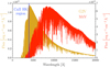Fig. 1 Model G2V spectra (yellow) and model M4V spectra (red). The flux scale of the G2V is displayed on the left, and the flux scale of the M4V is given on the right. The blue shaded area indicates the region of the Ca II H and K lines.

2 Overview of the measurement equations

2.1 Mount Wilson S-index

The HKP-2 spectrophotometer installed at the Mount Wilson Observatory measures the Ca II H and K line cores with a triangular 1.09 Å full width at half maximum (FWHM) bandpass while simultaneously measuring two 20 Å wide bands; R, centered on 4001.07 Å, and V, centered on 3901.07 Å. To mimic the response of this instrument, Duncan et al. (1991) prescribed the following S index formula: $$S=8\alpha \frac{N_{\text{H}}+N_{\text{K}}}{N_R+N_V},$$(1)

where N_H, N_K, N_R, and N_V are the counts in their respective bands, and α is a proportionality constant equating measurements made by the HKP-2 spectrophotometer to those made with HKP-1; Duncan et al. (1991) adopted the value α = 2.4. The factor of 8 arises from the 8:1 duty cycle between the line core and continuum bandpasses. Since its inception, the S-index has been the most widely used activity indicator for FGK stars.

2.2 Chromospheric Ca II H and K ratio

To convert the dimensionless S_MWO into arbitrary surface flux F_HK, Middelkoop (1982) and Rutten (1984) derived a continuum conversion factor C_cf. The arbitrary surface flux is defined as $$F_{\text{HK}}=S_{\text{MWO}}{C}_{\text{cf}}{T}_{\text{eff}}^4{10}^{-14},$$(2)

and its conversion into absolute units is given by $${ℱ}_{\text{HK}}=K{F}_{\text{HK}},$$(3)

where ℱ_HK and K are in units of erg cm⁻² s⁻¹. $$R_{\text{HK}}^{{}^{\prime }}=\frac{{ℱ}_{\text{H}}^{{}^{\prime }}+{ℱ}_{\text{K}}^{{}^{\prime }}}{\sigma T_{\text{eff}}^4}=\frac{{ℱ}_{\text{HK}}^{{}^{\prime }}}{{ℱ}_{\text{bol}}},$$(4)

where ${ℱ}_{\text{H}}^{\prime }={ℱ}_{\text{H}}-{ℱ}_{\text{H,phot}}$ and ${ℱ}_{\text{K}}^{\prime }={ℱ}_{\text{K}}-{ℱ}_{\text{K,phot}}$. Here, ${ℱ}_{\text{H}}^{\prime }$ and ${ℱ}_{\text{K}}^{\prime }$ are the chromospheric fluxes, ℱ_H and ℱ_K are the surface fluxes, and ℱ_Hphot and ℱ_Kphot are the photospheric fluxes of the Ca II H and K lines, respectively. From a slight rearranging, Eq. (4) can be written as $$R_{\text{HK}}^{{}^{\prime }}=\frac{{ℱ}_{\text{HK}}-{ℱ}_{\text{HK,phot}}}{\sigma T_{\text{eff}}^4}=R_{\text{HK}}-R_{\text{HK,phot}},$$(5)

with the surface flux ratio given by $$R_{\text{HK}}=\frac{{ℱ}_{\text{HK}}}{\sigma T_{\text{eff}}^4}$$(6)

and the photospheric flux ratio given by $$R_{\text{HK,phot}}=\frac{{ℱ}_{\text{HK,phot}}}{\sigma T_{\text{eff}}^4}.$$(7)

Typically, $R_{\text{HK}}^{\prime }$ is measured through a conversion from the Mount Wilson S-index. The method pioneered by Noyes et al. (1984) calculates R_HK using the equation $$R_{\text{HK}}=1.34\times {10}^{-4}{C}_{\text{cf}}{S}_{\text{MWO}}.$$(8)

The quantity C_cf is a color-dependent conversion factor to remove the color-dependence of the S_MWO, and Noyes et al. (1984) used the Middelkoop (1982) relation, $$\log C_{\text{cf}}=1.13{\left(B-V\right)}^3-3.91{\left(B-V\right)}^2+2.84\left(B-V\right)-0.47,$$(9)

for 0.45 ≤ (B – V) ≤ 1.50. To calculate R_phot, Noyes et al. (1984) used the following relation: $$\log R_{\text{phot,N84}}=-4.898+1.918{\left(B-V\right)}^2-2.893{\left(B-V\right)}^3$$(10)

for 0.44 ≤ (B – V) ≤ 0.82. Equations (8) and (10) are then combined to obtain the chromospheric flux excess, $$R_{\text{HK}}^{{}^{\prime }}=R_{\text{HK}}-R_{\text{phot,N84}}.$$(11)

2.3 H-alpha

Hα can be measured in a similar way to R_HK in Eq. (4), but substituting Hα for Ca II H and K. The chromospheric flux ratio of Hα might be defined as the surface flux subtracted by the photospheric flux, divided by the bolometric flux so that $$\frac{{ℱ}_{\text{H}\alpha }^{{}^{\prime }}}{{ℱ}_{\text{bol}}}=\frac{{ℱ}_{\text{H}\alpha }-{ℱ}_{\text{H}\alpha ,\text{phot}}}{\sigma T_{\text{eff}}^4}.$$(12)

In brief, we measure the surface flux of each line, ℱ_line by integrating the flux of the template spectrum, normalized to a stellar atmosphere model, inside an integration window centered on the line core. We measure the photospheric flux, ℱ_line,phot, by integrating the flux of the stellar atmosphere model, with the same integration window centered on the line core. The bolometric flux ℱ_bol is determined from T_eff, which is needed to obtain a proper stellar atmosphere model for a given star. We provide more detail in Sect. 3.

3 Case study: HARPS M dwarf sample

We used high-resolution archival spectra obtained with the HARPS spectrograph (Pepe et al. 2002) installed on ESO’s 3.6 m telescope in La Silla, Chile. The sample mainly consists of 102 targets from the HARPS GTO M dwarf sample (Bonfils et al. 2013)¹. We also used data obtained for the Cool Tiny Beats survey (Anglada-Escudé et al. 2014; Berdinas et al. 2015)², which adds the following four stars to the sample: GJ 160.2, GJ 180, GJ 570B, and GJ 317. Last, the following six M dwarfs with published planetary systems, and that are available in the ESO HARPS public archive, were added: GJ 676A, GJ 1214, HIP 12961, GJ 163, GJ 3634, and GJ 3740. Photometry values, mean radial velocities, proper motions, and parallaxes were acquired from SIMBAD (Wenger et al. 2000; see Table D.1).

3.1 High S/N template spectra

We used the HARPS-TERRA software (Anglada-Escudé & Butler 2012) for all available spectra on all stars in the sample. HARPS-TERRA is a sophisticated tool that matches individual spectra to a high S/N “template spectrum” using a least-squares fit to compute high-precision radial velocities. The high S/N template spectrum is obtained by coadding all individual spectra of a given star using the highest S/N spectrum as a basis spectrum. Pixel weighting, telluric masking, and outlier filtering are all implemented in the algorithm to assess and reduce systematic biases (see Sect. 2 in Anglada-Escudé & Butler 2012 for a much more detailed explanation). Because of this technique, the template spectrum for a star is essentially an averaged spectrum with median clipping. For each star, we obtained a high S/N template spectrum of each spectral order. We then used the corresponding spectral order that contains the chromospheric line of interest as the stellar observation spectrum.

After the initial run of HARPS-TERRA on all spectra of each target, we ran HARPS-TERRA a second time, excluding spectra that matched any of the following criteria: (1) program ID 60.A-9036(A), where spectra were acquired under nonoptimal conditions (an engineering run), (2) spectra reduced with cross-correlation function (CCF) masks earlier than M2 (the HARPS DRS pipeline uses an M2 mask for all M stars), and (3) spectra with radial velocity (RV) outliers determined by inspection. In general, looking at the RV time-series, spurious observation differences on the order of 1–10 km s⁻¹ with respect to most observations are considered outliers. All three of the above criteria could negatively influence the resulting template spectra in a suboptimal way. After the second run of HARPS-TERRA, we corrected for the blaze function by running HARPS-TERRA a third time with the -useblaze option and the blaze file given by the ESO DRS BLAZE FILE keyword in the template spectrum file header. Finally, we obtained a blaze-corrected high S/N template spectrum for each star.

3.2 Photospheric flux from stellar atmosphere models

To calculate photospheric fluxes, we used a grid of PHOENIX-ACES stellar atmosphere models from the Göttingen Spectral Library³ (Husser et al. 2013). The parameters and step sizes of the grid are listed in Table 1. We calculated ℱ_{HK, phot} by setting a 1.09 Å FWHM triangular bandpass centered on the Ca II H and K lines and summing the flux. The triangular bandpass mimics the response of the H and K bands of the HKP-2 Mount Wilson spectrograph (Duncan et al. 1991: see Sect. 2.1). To measure the fractional chromospheric flux ${ℱ}_{\text{H}\alpha }^{\prime }/{ℱ}_{\text{bol}}$, we used a 5.0 Å wide rectangular bandpass centered on Hα.

3.3 Surface flux from a high S/N template spectum

For a given star, the surface flux is measured from the high S/N template spectrum computed in Sect. 3.1. In the left panel of Fig. 2, we plot a single HARPS observation of the Ca II K line of an M 1.5 star. Because HARPS has a high resolution of R ~ 110 000, the S/N in the region near the calcium line is low, as shown in the figure. The right panel of Fig. 2 shows the same line of the same star, but this time, with 47 observations coadded together. This demonstrates the considerable S/N improvement obtained by coadding spectra.

For a single chromospheric line of a given star, the entire template order spectrum is normalized to a PHOENIX model spectrum via a first-degree polynomial least-squares fit, namely ℱ(λ) = af (λ) + b. The PHOENIX spectra were bilinearly interpolated to a precision of ΔT_eff = 1K and Δ[Fe/H] = 0.01 dex using the stellar parameters chosen by the methods outlined in Sect. 3.5 and listed in Table D.2. For the Ca II K line, we used order 6, for the Ca II H line, we used order 8, and for Hα, we used order 68. Before normalizing the template spectrum to the PHOENIX spectrum, we converted counts into energy, shifted the spectrum to rest wavelengths, and then transformed wavelengths to vacuum wavelengths. We masked the active lines, as well as Hϵ at 3971.2 Å. To reduce the influence of low S/N at the spectral order edges from the blaze function, we also masked the outer 10% of each order. We took the sum of the line flux in the same manner as in Sect. 3.2.

Figure 3 demonstrates this normalization of a high S/N template spectrum of an early-M dwarf normalized to a PHOENIX atmosphere model around the Ca II K line. The high S/N template spectrum consists of all available spectra coadded and flux-calibrated to the PHOENIX model atmosphere. Similarly, Fig. 4 shows this normalization of an M dwarf with Hα in absorption, while Fig. 5 shows another M dwarf with Hα in emission.

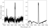Fig. 2 Ca II K line of an M1.5 star. Left: spectrum of a single HARPS observation. Right: template spectrum consisting of 47 coadded spectra of the same star.

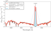Fig. 3 High S/N template spectrum of an early-M dwarf normalized to a PHOENIX atmosphere model. The solid red line is the high S/N template spectrum, while the dashed black line is the PHOENIX model atmosphere. The blue shaded region shows the chromospheric emission. The dotted lines indicate the 1.09 Å FWHM triangular bandpass used to integrate the Ca II H and K lines.

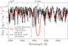Fig. 4 High S/N template spectrum of an M dwarf with Hα in absorption normalized to a PHOENIX atmosphere model. The solid red line is the high S/N template spectrum, while the dashed black line is the PHOENIX model atmosphere. The vertical dotted lines indicate a 5.0 Å integration region.

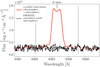Fig. 5 High S/N template spectrum of an active M dwarf with Hα in emission normalized to a PHOENIX atmosphere model. The solid red line is the high S/N template spectrum, while the dashed black line is the PHOENIX model atmosphere. The vertical dotted lines indicate the 5.0 Å integration region of Hα.

3.4 S-index comparison

As a sanity check, we compared the S -index values of our sample (for their values, we refer to Boro Saikia et al. 2018 and for the treatment of how they were calculated) with those of Astudillo-Defru et al. (2017) in Fig. 6. Although it agrees, the linear fit slightly overestimates the values of Astudillo-Defru et al. (2017) compared to Boro Saikia et al. (2018) for S values below 2, $$S_{\text{AD17}}=1.0487S_{\text{BS18}}+0.008$$(13)

3.5 Stellar parameters

For an accurate stellar atmosphere model to normalize a template spectrum to, we must first determine a set of stellar parameters for each star in a self-consistent manner. Here we describe the different calibrations we used to determine effective temperature and how we determined metallicity.

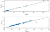Fig. 6 SAD17 of Astudillo-Defru et al. (2017) vs our work SBS18 (Boro Saikia et al. 2018). Top: entire range of the sample. Bottom: same sample with zoomed in axes. The dotted line shows the 1:1 relation.

Effective temperature

For each star in the sample, we estimated T_eff using three different calibrations. The first and second calibration used the combined relation of spectral type, effective temperature, mass, and radius from Kenyon & Hartmann (1995) and Golimowski et al. (2004). This same combination of calibrations was used by Reiners & Basri (2007), Shulyak et al. (2011), and Reiners & Mohanty (2012). The first method simply converts spectral type into effective temperature. We denote effective temperatures obtained from this method with T_{eff, SpT}. The second method uses the $M_{K_S}-{ℳ}_{\star }$ calibration of Delfosse et al. (2000) to first obtain a mass ℳ_⋆ from the absolute $M_{K_S}$ magnitude, and then uses the former relation to convert ℳ_⋆ into T_eff. We denote effective temperatures obtained from this method with $T_{\text{eff,}{ℳ}_{\star }}$. The third method adopts T_eff values obtained by Maldonado et al. (2015) of 53 stars in the HARPS M dwarf GTO sample. We denote effective temperatures from this study with T_{eff, M15}.

Metallicity

Maldonado et al. (2015) also calculated metal-licities of the same 53 targets using the pseudo-equivalent width (PEW) technique of Neves et al. (2014), who also calculated metallicities for the entire HARPS GTO M dwarf sample. Maldonado et al. (2015) reported that their results agreed well overall with those of Neves et al. (2014), and we therefore adopted the metallicities of Neves et al. (2014) for the sample completeness. Although effective temperatures were also calculated, the authors noted that their T_eff values are systematically underestimated compared with other works; therefore, we did not adopt the T_eff values of Neves et al. (2014). For two stars not listed in Neves et al. (2014, GJ 570B and GJ 180), we used the conversion of $M_{K_S}$ and V – K to [Fe/H] in Neves et al. (2012). We note that the difference in metallicities between Neves et al. (2012) and Maldonado et al. (2015) can be up to Δ[Fe/H] ± 0.2. However, this difference is much smaller than the resolution of our grid of models, Δ[Fe/H] ± 0.5. For stars with no $M_{K_S}$ or V – K_S measurements, we assumed solar metallicity. For all stars in the sample, we constrained the surface gravity to log(ɡ) = 5.0, which is a typical value for M dwarfs. The stellar parameters we used are listed in Table D.2.

The top panel of Fig. 7 shows T_eff of the three methods we used as a function of $M_{K_S}$, with their metallicity represented by color. For T_eff,SpT, we were able to calibrate 110 stars. With $T_{\text{eff,}{ℳ}_{\star }}$, we were able to calibrate 99 stars, and for T_eff,M15, there are 49 stars. Temperatures of the same star are connected with a solid vertical line. In the lower panel of Fig. 7, we show the residuals of the different sources of T_eff. As is evident from both panels, the T_eff determined by different methods disagrees to some extent, and this becomes much more pronounced for stars with $M_{K_S}>8$. The mean of all ΔT_eff values is 176 K. For ΔT_eff values with $M_{K_S}<8$, the mean difference drops to 122 K. The mean of ΔT_eff values for $M_{K_S}>8$ increases to 363 K. Most of these values with $M_{K_S}>8$ belong to $T_{\text{eff,}{ℳ}_{\star }}-T_{\text{eff,SpT}}$.

We note that metallicity has an effect on the T_eff determination. The largest scatter in ΔT_eff is between T_eff,SpT and T_eff,M15. The determination of the spectral type depends on line ratios that are sensitive to both T_eff and [Fe/H]. Moreover, Maldonado et al. (2015) determined T_eff simultaneously with metallicity, However, metallicity does not have much impact when determining T_eff from $M_{K_S}-{ℳ}_{\star }$, as infrared absolute magnitudes are less sensitive to metallicity (Delfosse et al. 2000). For $T_{\text{eff,}{ℳ}_{\star }}$, since ℳ_⋆ is determined from a polynomial as a function of $M_{K_S}$, we expect to see a clear relation between T_eff and $M_{K_S}$. Whether $M_{K_S}$ actually is such a precise indicator of T_eff is beyond the context of this study. Regardless, accurate effective temperatures of M dwarfs remain elusive; see Mann et al. (2015) and Passegger et al. (2016) for more thorough analyses of the current state of M dwarf stellar parameter determination.

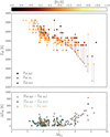Fig. 7 Effective temperature Teff of the stellar sample using different Teff determination methods, which are shown by different plot symbols. Top: effective temperature Teff as a function of absolute magnitude $M_{K_S}$ with metallicity [Fe/H] shown according to the color scale. Temperatures of the same star are connected with a solid vertical line. Bottom: difference of the methods used to obtain Teff in K.

4 Results

4.1 Chromospheric Ca II H and K flux

We plot the chromospheric Ca II H and K flux normalized to bolometric flux, log $R_{\text{HK}}^{{}^{\prime }}$, as a function of absolute magnitude $M_{K_S}$ in Fig. 8. log $R_{\text{HK}}^{{}^{\prime }}$ was calculated using the spectral subtraction technique outlined in Sect. 3, following Eq. (4). We estimated T_eff using the three different methods described in Sect. 3.5 and for each T_eff, calculated log $R_{\text{HK}}^{{}^{\prime }}$. The plot legend contains the colors of each T_eff calibration. We connect log $R_{\text{HK}}^{{}^{\prime }}$ measurements of the same star but different effective temperatures with a solid vertical line. Additionally, we plot stars with known planetary systems with open symbols, and stars without known planetary systems with closed symbols. Stars without Hα in emission are plotted with a circle and stars exhibiting Hα emission with a triangle.

4.1.1 T_eff,SpT calibration

For 110 stars we have spectral type information and are able to measure log $R_{\text{HK}}^{{}^{\prime }}$ using the spectral type to T_eff conversion, T_eff,SpT. Of these stars, 13 exhibit Hα emission, and 19 have known planetary systems. The earliest-M dwarfs with $M_{K_S}<5.8$ have higher values of log $R_{\text{HK}}^{{}^{\prime }}$, between –4.8 and –4.5. There is a drop in the lower boundary of activity levels near $M_{K_S}=5.7$, where values range from –5.3 < log $R_{\text{HK}}^{\prime }$. After this drop, the sequence of lower-activity stars has no apparent drop, and log $R_{\text{HK}}^{\prime }$ stays between –5.5 and –4.9. Stars exhibiting Hα emission tend to have much higher log $R_{\text{HK}}^{\prime }$ values than those that do not exhibit Hα emission. Their measured activity levels are log $R_{\text{HK}}^{\prime }>-4.7$ and can be as high as log $R_{\text{HK}}^{\prime }=-3.8$.

4.1.2 $T_{\text{eff,}{ℳ}_{★}}$ calibration

For 99 stars, we have $M_{K_S}$ measurements and can measure log $R_{\text{HK}}^{\prime }$ using the $M_{K_S}$ to mass to T_eff calibration $T_{\text{eff,}{ℳ}_{★}}$. Of these stars, 13 exhibit Hα emission, and 16 have known planetary systems. Unlike log $R_{\text{HK}}^{\prime }$ measured with T_{eff, SpT}, the lower boundary of activity for $T_{\text{eff,}{ℳ}_{★}}$ decreases with $M_{K_S}$. This relation is expected because in this case, $T_{\text{eff,}{ℳ}_{★}}$ is calibrated using $M_{K_S}$. This does not have a dramatic effect on log $R_{\text{HK}}^{\prime }$ values until $M_{K_S}=8$. At higher $M_{K_S}$, the difference in log $R_{\text{HK}}^{\prime }$ can be as high as 1.3 dex, and this arises from the large differences in T_eff seen in Fig. 7. However, even though the measured values of log $R_{\text{HK}}^{\prime }$ using $T_{\text{eff,}{ℳ}_{★}}$ are much lower, stars with Hα in emission still have significantly higher log $R_{\text{HK}}^{\prime }$ values than their counterparts.

4.1.3 T_eff,M15 calibration

For 49 stars with adopted values from Maldonado et al. (2015), we are able to measure log $R_{\text{HK}}^{\prime }$ using T_eff,M15. Of these stars, 4 exhibit Hα emission, and 9 have known planetary systems. Similar with the other T_eff calibrations, the lower level of log $R_{\text{HK}}^{\prime }$ decreases from −4.5 to −5.4 between $5<M_{K_S}<6.4$. There are only three stars with $M_{K_s}\gtrsim 8$, and they tend to agree more with T_eff,SpT values than $T_{\text{eff,}{ℳ}_{*}}$.

We list the individual log ${R^{\prime }}_{\text{HK}}$ measurements in Table D.3. The largest differences of log ${R^{\prime }}_{\text{HK}}$ values occur at the latest spectral types where it is difficult to determine a consistent T_eff using a color, magnitude, or spectral type relation. For the entire sequence of stars, the mean of ${R^{\prime }}_{\text{HK}}$ is 0.17 dex. At $M_{K_S}<8$, the mean of ${R^{\prime }}_{\text{HK}}$ is only 0.10 dex, however for $M_{K_S}>8$, the mean is 0.56 dex. The star with the highest difference in log ${R^{\prime }}_{\text{HK}}$ is GJ 1002, which has $\Delta \log {R^{\prime }}_{\text{HK}}=1.31$ dex. This is because of its wide range of T_eff calibrations, with ΔT_eff = 534 K.

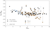Fig. 8 Fractional chromospheric Ca II H and K flux normalized to bolometric flux on a logarithmic scale, log ${R^{\prime }}_{\text{HK}}$, as a function of absolute magnitude $M_{K_S}$. For each star, log ${R^{\prime }}_{\text{HK}}$ is calculated with different Teff calibrations, each plotted with a different color. Vertical gray lines connect different measurements of the same star. Triangles indicate stars exhibiting Hα emission. Filled symbols indicate stars without known planetary systems, and open symbols indicate stars with known planetary systems.

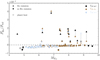Fig. 9 Fractional chromospheric Ha flux, ${{ℱ}^{\prime }}_{\text{Hα}}/{ℱ}_{\text{bol}}$, as a function of absolute magnitude $M_{K_S}$. Vertical gray lines connect different measurements of the same star. Triangles indicate stars exhibiting Hα emission. Filled symbols indicate stars without known planetary systems, and open symbols indicate stars with known planetary systems. Values >0 indicate that Hα is in emission, and values <0 indicate that Hα is in absorption. Values near 0 indicate filling-in of the line to the continuum.

4.2 Chromospheric H-alpha flux

In Fig. 9, we correct for the photospheric contribution and plot the chromospheric flux ratio of Hα, ${{ℱ}^{\prime }}_{\text{Hα}}/{ℱ}_{\text{bol}}$. This is not on a logarithmic scale, unlike how we plot log ${R^{\prime }}_{\text{HK}}$. This is because the sign of ${{ℱ}^{\prime }}_{\text{Hα}}/{ℱ}_{\text{bol}}$ indicates whether the line is in emission or absorption. Values of ${{ℱ}^{\prime }}_{\text{Hα}}/{ℱ}_{\text{bol}}~0$ indicate that Ha is filled to the continuum. Values ${{ℱ}^{\prime }}_{\text{Hα}}/{ℱ}_{\text{bol}}>0$ indicate that Ha is in emission, as in Fig. 5, while values ${{ℱ}^{\prime }}_{\text{Hα}}/{ℱ}_{\text{bol}}<0$ indicate that Hα is in absorption as in Fig. 4. The plotting colors and symbols are the same as used in Fig. 8.

For stars with Ha in absorption, ${{ℱ}^{\prime }}_{\text{Hα}}/{ℱ}_{\text{bol}}$ increases toward a filling-in of the continuum toward larger $M_{K_S}$. The stars in which Hα is in emission tend to have significantly higher ${{ℱ}^{\prime }}_{\text{Hα}}/{ℱ}_{\text{bol}}$ than stars for which Hα is near the continuum level. We note that the absorption of Ha stays in a relatively narrow range. Values of ${{ℱ}^{\prime }}_{\text{Hα}}/{ℱ}_{\text{bol}}$ are $-0.6\times {10}^{-4}<{{ℱ}^{\prime }}_{\text{H}\alpha }/{ℱ}_{\text{bol}}\lesssim 0$. However, for stars in which Hα is in emission, the range of ${{ℱ}^{\prime }}_{\text{H}\alpha }/{ℱ}_{\text{bol}}$ is on the order of several 10⁻⁴. larger $\Delta {{ℱ}^{\prime }}_{\text{H}\alpha }/{ℱ}_{\text{bol}}$ due to the different T_eff calibrations. Stars for which Hα is in emission also have significantly higher values of ${R^{\prime }}_{\text{HK}}$ than those in which Hα is not in emission.

4.3 H-alpha versus calcium II H and K flux

We plot chromospheric flux values of Hα against Ca II H and K in Figs. 10 and 11. Figure 10 contains flux in absolute flux units, and therefore contains negative values of Hα that correspond to absorption. Figure 11 shows flux on a log-scale and excludes inactive stars with Hα in absorption. Symbols and markers are the same as in Figs. 8 and 9.

Figure 10 shows Hα only in absoprtion $\left({{ℱ}^{\prime }}_{\text{Hα}}\lesssim 0\right)$, and a decreasing trend is apparent where it goes deeper into absorption with increasing ${{ℱ}^{\prime }}_{\text{HK}}$. The trend appears to be linear from $0.0\le {{ℱ}^{\prime }}_{\text{HK}}\le 4.0\times {10}^{-5}$ erg cm⁻² s⁻¹. When Hα is in emission, the trend of ${{ℱ}^{\prime }}_{\text{Hα}}$ increases with increasing ${{ℱ}^{\prime }}_{\text{HK}}$. This deepening of the Hα line before filling-in and going into emission was reported by Walkowicz & Hawley (2009) and Scandariato et al. (2017). Scandariato et al. (2017) only observed a decreasing trend from $0.0\le {{ℱ}^{\prime }}_{\text{HK}}\le 1.0$. In Fig. 11, we overplot as a dashed red line a linear fit that we find to be $$\log {ℱ}_{\text{H}\alpha }^{{}^{\prime }}=0.7571\log {ℱ}_{\text{HK}}^{{}^{\prime }}+1.6695,$$(14)

with R² = 0.706.

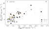Fig. 10 Fractional chromospheric Hα flux, ${{ℱ}^{\prime }}_{\text{Hα}}$, as a function of fractional chromospheric Ca II H and K flux, ${{ℱ}^{\prime }}_{\text{HK}}$ flux. Filled symbols indicate stars without known planetary systems, and open symbols indicate stars with known planetary systems. Values >0 indicate that Hα is in emission, and values <0 indicate that Hα is in absorption. Values near 0 indicate filling-in of the line to the continuum.

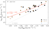Fig. 11 Fractional chromospheric Hα flux, ${{ℱ}^{\prime }}_{\text{Hα}}$, as a function of fractional chromospheric Ca II H and K flux, ${{ℱ}^{\prime }}_{\text{HK}}$ flux, both on a logarithmic scale. Filled symbols indicate stars without known planetary systems, and open symbols indicate stars with known planetary systems. In this plot, only stars with Hα in emission (>0) are shown. A linear fit is shown with a dashed red line, and a 1:1 relation is plotted as a dotted gray line.

4.4 Ca II H and K surface flux calibrations

We compared calibrations of the continuum conversion factor C_cf (used for measuring F_HK) of other studies with C_cf calibrations using the PHOENIX model grid. To derive our T_eff dependent conversion factor C_cf, we combined Eqs. (2), (3), and $S=8\alpha \left({ℱ}_{\text{HK}}/{ℱ}_{RV}\right)$, to arrive at $$C_{\text{cf}}=\frac{{10}^{14}}{8\alpha K}\frac{{ℱ}_{\text{RV}}}{T_{\text{eff}}^4}.$$(15)

Using values of α = 2.4 and K = 1.07 × 10⁶ erg cm⁻² s⁻¹ (Hall et al. 2007), we then obtained $$C_{\text{cf}}=4.8676\times {10}^6\cdot \frac{{ℱ}_{\text{RV}}}{T_{\text{eff}}^4}.$$(16)

The top panel of Fig. 12 shows our computed log C_cf as a function of T_eff. Different values of [Fe/H] are shown as a function of color, and different values of log(ɡ) are plotted with different symbols. For T_eff > 5000 K, we used log(ɡ) values of 4.0 and 4.5, and for T_eff ≤ 5000 K, we used log(ɡ) values of 4.5 and 5.0. A fifth-order polynomial, $$\log C_{\text{cf}}=a+b{T}_{\text{eff}}+c{T}_{\text{eff}}{}^2+d{T}_{\text{eff}}{}^3+e{T}_{\text{eff}}{}^4+f{T}_{\text{eff}}{}^5,$$(17)

was fit to all of the points and overplotted as a solid red line. The coefficients of this polynomial are listed in Table 2. We provide the computed PHOENIX stellar atmosphere log C_cf values in Table D.4 for the entire model grid.

Even for the wide range of metallicity values, the spread of log C_cf is not too wide for T_eff > 3400 K. For these higher temperatures, log C_cf varies by 0.25 dex at most. At T_eff < 3100 K, metallicity begins to contribute to a larger spread of log C_cf values, around 0.5 dex. This spread of log C_cf increases to 1.4 dex as T_eff decreases to 2300 K.

The bottom panel of Fig. 12 compares the polynomial fit in the upper panel with previously published log C_cf-T_eff relations (see Appendix A for details about the relations).

For the relations of the other authors, we plot the range for which the relations are calibrated. Our log C_cf values agree well with those from other studies for T_eff ≳ 4100 K to ~0.1 dex. At temperatures cooler than 4100 K, our log C_cf values start to deviate from those of Middelkoop (1982); Rutten (1984); Cincunegui et al. (2007); Suárez Mascareño et al. (2015); and Astudillo-Defru et al. (2017); our values are higher for cooler temperatures. For temperatures cooler than T_eff = 4100 K, log C_cf diverges by more than 0.2 dex. The difference between our relation and Cincunegui et al. (2007) increases to 0.4 dex at T_eff = 3100 K, while the difference between our relation and both Suárez Mascareño et al. (2015) and Astudillo-Defru et al. (2017) increases to 0.8 dex at T_eff = 3000 K. This discrepency in log C_cf might be attributed to the use of empirical calibrations with these studies as opposed to this work using stellar models (see Sect. 5).

As an example, when we take for the Sun B – V = 0.642 and S_MWO = 0.164, the Noyes et al. (1984) calibration of R_HK will give us log R_HK = −4.62. Our calibration using Eq. (17) results in log R_HK = −4.60. This means that for a Sun-like star, Δ log R_HK = 0.02.

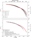Fig. 12 Different log Ccf calibrations as a function of Teff. The approximate spectral type is shown on the top axis. Top: PHOENIX stellar atmosphere models with different [Fe/H] and log(ɡ), where [Fe/H] is indicated by color and log(ɡ) indicated by symbol. The solid red line indicates a fifth-order polynomial fit. Bottom: calibrations of log Ccf from other works where only the valid calibration region is plotted. Overplotted in red is the same fifth-order polynomial fit from the top panel.

4.5 Ca II H and K photospheric flux calibrations

In the top panel of Fig. 13, we plot log R_HK,phot as a function of T_eff, computed as described in Sect. 3.2. The colors and symbols are assigned in the same manner as in Fig. 12. A fifth-order polynomial fit $$\log R_{\text{HK,phot}}=a+b{T}_{\text{eff}}+c{T}_{\text{eff}}{}^2+d{T}_{\text{eff}}{}^3+e{T}_{\text{eff}}{}^4+f{T}_{\text{eff}}{}^5,$$(18)

is overplotted as a solid red line, and coefficients of this polynomial are listed in Table 3. Similarly as with log C_cf, metallicity has an effect on the spread of log R_HK,phot values. The spread increases at 4000 ≤ T_eff ≤ 5100 K and T_eff ≤ 3800 K. At T_eff > 5100 K, the spread of log R_HK,phot values is lower than 0.2 dex. The spread increases from T_eff = 5100 K to T_eff = 4200 K, where it is about 0.4 dex. At T_eff = 3100 K, the spread of log R_HK,phot is 0.6 dex. Here, a change in metallicity of ±0.5 dex can result in a Δ log R_HK,phot ~ 0.1 dex. At T_eff < 3300 K, the spread continually increases with lower temperatures to almost 1.6 dex at T_eff = 2400 K. At T_eff = 2400 K., a change in metal-licity of ±0.5 can result in a Δ log R_HK,phot ~ 0.5 dex. We provide the computed PHOENIX stellar atmosphere log R_HK,phot values in Table D.4 for the entire model grid.

In the bottom panel of Fig. 13, we compare our log R_HK,phot-T_eff polynomial fit with previous literature relations (see Appendix B for details about the relations). The higher log R_HK,phot values of both Mittag et al. (2013) and our work in comparison with Noyes et al. (1984) and Suárez Mascareño et al. (2015) are clear. The difference between Mittag et al. (2013) and Noyes et al. (1984) is ~0.3 dex, and the difference between our work and Noyes et al. (1984) ranges from 0.4 to 0.5 dex. The difference between our work and Suárez Mascareño et al. (2015) can be as large as 1.3 dex at T_eff = 3000 K. Our values of log R_HK,phot agree very well with those of Astudillo-Defru et al. (2017), with the largest difference being 0.12 dex at T_eff = 4800 K, and other differences on the order of 0.1 dex at T_eff = 3500,3400, and 3100 K.

Our log R_HK,phot calibration has much higher values than the calibration used by Noyes et al. (1984). This systematic offset was also observed by Astudillo-Defru et al. (2017), who also used synthetic spectra to obtain an R_HK,phot calibration. While the exact reason for this offset is not known (see the discussion in Astudillo-Defru et al. 2017), an offset correction can be applied to scale our log R_HK,phot calibration to Noyes et al. (1984), $$\log R_{\text{phot,N84}}=\log R_{\text{phot,ours}}-0.4612,$$(19)

where 0.4612 is the offset correction. This simple offset correction scales our log R_{HK phot} values to Noyes et al. (1984) values in their valid calibration region, so that our calibration can be used to obtain comparable results to Noyes et al. (1984), and also to extend the calibration to later-type stars. We note that although they are widely used, the Noyes et al. (1984) calibrations are only calibrated in the range 5300 K ≲ T_eff ≲ 6300 K.

If we take the same B – V and S_MWO values as in Sect. 4.4, the Noyes et al. (1984) calibration of R_{HK phot} will give us log R_{HK phot} = −4.92. This will give us an activity measurement of log ${R^{\prime }}_{\text{HK}}=-4.92$. Our calibration using Eq. (19) results in^log R_{HK, phot} = −4.89, which gives us log ${R^{\prime }}_{\text{HK}}=-4.91$. Then, for a Sun-like star, Δ log R_{HK phot} = 0.03 and $\Delta \log {R^{\prime }}_{\text{HK}}=0.01$.

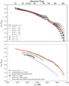Fig. 13 Different log RHK,phot as a function of Teff. The approximate spectral type is shown on the top axis. Top: PHOENIX stellar atmosphere models with different [Fe/H] and log(ɡ), where [Fe/H] is indicated by color and log(ɡ) indicated by symbol. The solid red line indicates a fifth-order polynomial fit. Bottom: calibrations of log RHK,phot from other works where only the valid calibration region is plotted. Overplotted in red is the same fifth-order polynomial fit from the top panel.

4.6 χ-factor

The χ-factor provides a method to convert the equivalent width of Ca II H and K into R_HK and Ha indto ${ℱ}_{\text{H}\alpha }/{ℱ}_{\text{bol}}$ in M dwarfs. Walkowicz et al. (2004) define the χ factor as the ratio of the Hα line continuum luminosity to bolometric luminosity, namely $$\chi =L_{\text{H}\alpha ,\text{cont}}/L_{\text{bol}},$$(20)

where L_Hα,cont is the luminosity of a selected continuum region near Hα. West & Hawley (2008) extend the selection of χ values to higher-order Balmer lines and Ca II H and K. When multiplied by the equivalent width of the respective line, we can obtain the ratio of the line luminosity to the bolometric luminosity, $$L_{\text{line}}/L_{\text{bol}}={\chi }_{\text{line}}\cdot {\text{EW}}_{\text{line}}.$$(21)

For both Ca II H and K and Hα, we calculated the χ values of West & Hawley (2008) of the PHOENIX model grid for M dwarf T_eff values and different metallicities, constraining log(ɡ) = 5.0. For Ca II H and K, we used the continuum regions given by Walkowicz & Hawley (2009), and for Hα, we used the continuum regions given by West & Hawley (2008). We plot these with the values listed in West & Hawley (2008) in Fig. 14, with Ca II H and K in the top panel and Hα in the lower panel. We provide the computed χ_line values in Table D.5.

Similar to Fig. 12, the continuum values diverge as T_eff decreases for different metallicities. For χ_CaIIHK, a metallicity of [Fe/H] = −0.5 agrees best with West & Hawley (2008). We note that all of our χ_CaIIHK values are higher for M3 and M4 spectral types. However, this difference is very small (on the order of 10⁻⁷), and the error bars of West & Hawley (2008) are much smaller than the spread of χ_CaIIHK by metallicity. Our χ Hα values also agree well with West & Hawley (2008), especially for [Fe/H] = 0.0. Our χ Hα values deviate from West & Hawley (2008) at spectral types M4 and earlier. However, like with χ_CaIIHK the difference is small, on the order of 10⁻⁶.

4.7 Proxima Centauri

Proxima Centauri, or GJ 551, is the only star in this study that exhibits Hα emission and is a known planet host (Anglada-Escudé et al. 2016). This indicator of high activity is consistent with the findings of Ribas et al. (2016), who reported that Proxima b receives ten times more far-UV flux than the current Earth.

Except for the T_eff,M15 calibration of Proxima Centauri ($\log {R^{\prime }}_{\text{HK}}=-3.92,T_{\text{eff,M15}}=3555\text{\hspace{0.17em}K}$), we did not measure log ${R^{\prime }}_{\text{HK}}>-4.5$ for any planet hosts. However, this particular value may be overestimated. For example, for Proxima Centauri, Boyajian et al. (2012) reported T_eff ~ 3050 K, and the calibration of T_eff,SpT = 2900 K, which has log ${R^{\prime }}_{\text{HK}}=-4.59$. The similarities between these two temperatures mean that log ${R^{\prime }}_{\text{HK}}$ of Proxima Centauri probably sits closer to approximately −4.5 than −3.9.

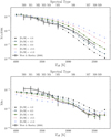Fig. 14 Top: continuum flux normalized to bolometric flux of Ca II H and K, χ Ca II HK, as a function of Teff using PHOENIX stellar atmospheres with log(ɡ) = 5.0 and different metallicities. Values from West & Hawley (2008) are plotted in gray. Bottom: continuum flux normalized to bolometric flux of Hα, χHα, as a function of Teff using PHOENIX stellar atmospheres with log(ɡ) = 5.0 and different metallicities. Values from West & Hawley (2008) are plotted in gray.

5 Discussion

With the exception of Proxima Centauri, which exhibits Hα in emission, the remaining known planet hosts exhibit low activity. This is expected as activity can mimic planetary signals and cause incorrect planet detections, so that stars with lower activity stars are preferred for planet searches.

There is a divergence of log C_cf values between our work and other works that begins at the start of the M dwarf sequence near 4000 K. Middelkoop (1982); Rutten (1984); Cincunegui et al. (2007); Suárez Mascareño et al. (2015), and Astudillo-Defru et al. (2017) used observational data to calibrate log C_cf as a function of B – V, while we used stellar models as a function of T_eff. The discrepency might be due to an insufficient (B – V) – T_eff relation in this region. However, our χ Ca II HK values agree with those of West & Hawley (2008), whose relations were also derived from observational data. This gives us confidence that the PHOENIX models are accurate in the continuum near the Ca II H and K lines, although the continuum region of χ Ca II HK differs from the region used in log C_cf.

Our log R_HK,phot values remain higher than log R_HK,phot values obtained using observational data (Noyes et al. 1984; Suárez Mascareño et al. 2016). As noted by Mittag et al. (2013), this difference arises from the integration region of the calcium line. Our work and Mittag et al. (2013) both integrated the entire photospheric line. The log R_HK,phot relation used by Noyes et al. (1984) is that of Hartmann et al. (1984), who only estimated the flux outside of the line core exterior to the H1 and K1 points: they assumed the flux of the line core to be zero. The log R_HK,phot relation derived by Suárez Mascareño et al. (2015) also masks the line core: 0.7 Å for FGK stars, and 0.4 Å for M stars. For this reason, we provide the correction factor in Eq. (19) to keep the calculated ${R^{\prime }}_{\text{HK}}$ values consistent with historical published measurements based on Noyes et al. (1984). Moreover, although both use PHOENIX models, our log R_{HK phot} values are still higher than those of Mittag et al. (2013). One reason for this difference might be the models that were used; Mittag et al. (2013) used models computed in non-local thermo-dynamic equilibrium, while we used models computed in local thermodynamic equilibrium.

Astudillo-Defru et al. (2017) measured ${R^{\prime }}_{\text{HK}}$ of 403 stars of the HARPS M dwarf sample. They extended the technique of Noyes et al. (1984) by calibrating their own log C_cf using 14 G or K and M dwarf pairs and use BT-Settl models to arrive at R_HK,phot through an S-index conversion. Although we used different methods to arrive at the measurement of ${R^{\prime }}_{\text{HK}}$ in M dwarfs, we find our results to be consistent with Astudillo-Defru et al. (2017). Namely, our Fig. 8 exhibits a very similar lower envelope of ${R^{\prime }}_{\text{HK}}$ values to their Fig. 10. For brighter $M_{K_S}$ values (earlier-M dwarf types), we find a relatively constant lower envelope of ${R^{\prime }}_{\text{HK}}$ values (see Fig. 8), while Astudillo-Defru et al. (2017) also reported a constant lower envelope of ${R^{\prime }}_{\text{HK}}$ for the higher M dwarf masses (see their lower Fig. 10). As $M_{K_S}$ increases and M dwarf types move to later types, the lower envelope of $R_{\text{HK}}^{\prime }$ values begins to decrease. Finally, this lower envelope flattens out again for lower masses, or later spectral types. Mittag et al. (2013) similarly reported that the initially constant lower envelope was followed by a decreasing lower envelope. We note a key difference in our findings in that the technique used to derive T_eff influences the extent of the decreasing lower envelope and then the level of the constant envelope for the lowest masses. However, each method individually still exhibits this behavior.

Surveys that focus on determining stellar parameters (e.g., Maldonado et al. 2015) would be the more reliable source of stellar parameters if the given star were included in that survey. Moreover, when the S-index of a given star is the sole measurement and no access to any spectra is possible, then we recommend the use of Eqs. (17) and (18) to calculate $R_{\text{HK}}^{\prime }$.

6 Summary and conclusions

In this work, we have measured Ca II H and K and Hα activity in a large sample of HARPS M dwarf spectra using high S/N template spectra and PHOENIX model atmospheres. We compared three different T_eff calibrations and find ΔT_eff ~ several 100 K for mid- to late-M dwarfs. This uncertainty in T_eff contributes up to Δ log $R_{\text{HK}}^{\prime }=1.31$ dex and Δ log ${{ℱ}^{\prime }}_{H\alpha }/{ℱ}_{\text{bol}}=2.93$ dex. We have extended $R_{\text{HK}}^{\prime }$ calibrations to the M dwarf regime using PHOENIX model spectra. We compared these new $R_{\text{HK}}^{\prime }$ calibrations with previous calibrations. Our log C_cf calibration agrees very well with previous calibrations within 0.2 dex, and extends the calibration from 3100 K ≤ T_eff ≤ 6800 K to 2300 K ≤ T_eff ≤ 7200 K. Our log R_HK,phot calibration overstimates the Noyes et al. (1984) calibration by 0.46 dex. However, our calibration extends log R_HK,phot to 2300 K ≤ T_eff ≤ 7200 K, and a simple offset correction can be applied to scale our log R_HK,phot to that of Noyes et al. (1984). We have provided a grid of log C_cf and log R_HK,phot values as functions of T_eff, [Fe/H], and log(ɡ). This grid can be used to compute $R_{\text{HK}}^{\prime }$ from S-index values using either polynomial fits to or an interpolation of the grid, and can be further beneficial when constraints on the stellar parameters of the targets are established. We have calculated χ_CaIIHK and χHα for −1.0 ≤ [Fe/H] ≤ +1.0 in steps of Δ [Fe/H] = 0.5 for the entire M dwarf T_eff range. We find that our χ values from PHOENIX models agree well with the χ values of West & Hawley (2008).

We find that the lower boundary of log $R_{\text{HK}}^{\prime }$ either stays constant or decreases with later-M dwarfs depending on the T_eff calibration used. Because of conflicting T_eff measurements toward later-M dwarfs, an accurate determination of $R_{\text{HK}}^{\prime }$ cannot be made beyond $M_{K_S}>8.$. For ${{ℱ}^{\prime }}_{H\alpha }/{ℱ}_{\text{bol}}$, the lower boundary of inactive stars begins with early-M dwarfs in deeper absorption, and fills in to the continuum towards later-M dwarfs. Stars with known planetary systems do not exhibit unexpected or peculiar levels of Ca II H, K, and Hα activity in relation to stars of similar spectral type or absolute magnitude.

Our surface flux calibration of log C_cf agrees very well with that of Middelkoop (1982) for FGK stars, and our surface flux calibrations of χ_CaIIHK and χHα also agree well with those of West & Hawley (2008) for M stars. Our $R_{\text{HK}}^{\prime }$ calibrations agree very well with those of Noyes et al. (1984) to within Δ log $R_{\text{HK}}^{\prime }=0.01$ dex for the Sun. We conclude that our calibrations are a reliable extension to previous $R_{\text{HK}}^{\prime }$ calibrations, provide a consistent way to measure $R_{\text{HK}}^{\prime }$ across spectral types early F to late M, and allow the comparison of activity of Sun-like stars to M dwarfs.

Acknowledgements

We thank Tim-Oliver Husser for fruitful discussions and providing us with recalculated PHOENIX models. The authors acknowledge research funding by the Deutsche Forschungsgemeinschaft (DFG) under the grant SFB 963, project A04. SVJ acknowledges the support of the DFG priority program SPP 1992 “Exploring the Diversity of Extrasolar Planets” (JE 701/5-1). SBS acknowledges the support of the Austrian Science Fund (FWF) Lise Meitner project M2829-N. This work is based on data products from observations made with ESO Telescopes at the La Silla Observatory (Chile) under the program IDs 60.A-9036, 072.C-0488, 074.C-0364, 075.C-0202, 075.D-0614, 076.C-0155, 077.C-0364, 078.C-0044, 082.C-0718, 085.C-0019, 086.C-0284, 087.C-0831, 089.C-0050, 089.C-0732, 090.C-0395, 090.C-0421, 091.C-0034, 180.C-0886, 183.C-0437, 183.C-0972, 185.D-0056, 191.C-0505, 192.C-0224, and 283.C-5022. We acknowledge the effort of all the observers of the aforementioned ESO projects whose data we have used.

Appendix A Ca II H and K surface flux calibrations

Measuring log C_cf of 85 main-sequence stars from the Vaughan & Preston (1980) survey of the solar neighborhood, Middelkoop (1982) fit a polynomial to log C_cf as a function of B – V, $$\log C_{\text{cf,M82}}=1.13{\left(B-V\right)}^3-3.91{\left(B-V\right)}^2+2.84\left(B-V\right)-0.47$$(A.1)

for 0.45 ≤ (B – V) ≤ 1.50.

Rutten (1984) extended the relation further by measuring 30 additional main-sequence stars and also 27 subgiants and giants, $$\log C_{\text{cf,R84}}=0.25{\left(B-V\right)}^3-1.33{\left(B-V\right)}^2+0.43\left(B-V\right)+0.24,$$(A.2)

which is valid for main-sequence stars with 0.3 ≤ (B – V) ≤ 1.6.

Cincunegui et al. (2007) extended the calibration using 109 stars ranging from spectral type F6 to M5, $$\log C_{\text{cf,CDM07}}=-0.33{\left(B-V\right)}^3-0.55{\left(B-V\right)}^2-1.41\left(B-V\right)+0.8$$(A.3)

for 0.45 ≤ (B – V) ≤ 1.81. Middelkoop (1982), Rutten (1984), and Cincunegui et al. (2007) all made use of the relation of Noyes et al. (1984) to convert B – V into T_eff.

Instead of using observational spectra, Mittag et al. (2013) used PHOENIX stellar atmosphere models to measure ℱ_RV directly in absolute flux units, $$\log {\left({ℱ}_{RV}/19.2\right)}_{\text{MSS13}}=8.33-1.79\left(B-\text{}V\right),$$(A.4)

where 0.44 ≤ (B – V) ≤ 1.60. They transformed this to log C_cf using $$\log C_{\text{cf}}=8.33-1.79\left(B-V\right)-\log \alpha -\log T_{\text{eff}}{}^4-14,$$(A.5)

where α = 19.2, and used the B – V to T_eff relation of Gray (2005).

Similarly, Pérez Martínez et al. (2014) also used PHOENIX models to derive a conversion factor $$\log C_{\text{cf,PMSH14}}=0.66-1.11\left(B-\text{}V\right)$$(A.6)

for 0.44 ≤ (B – V) ≤ 1.33. Pérez Martínez et al. (2014) used the B – V to T_eff tables of Schmidt-Kaler (1982) (which they also included in their publication).

Using HARPS spectra of FGKM stars, Suárez Mascareño et al. (2015) derived a continuum correction factor $$\begin{array}{l}\log C_{\text{cf,SM15}}=0.668-1.270\left(B-V\right)\hfill \\ +0.645{\left(B-V\right)}^2-0.443{\left(B-V\right)}^3\hfill \end{array}$$(A.7)

for 0.4 ≲ (B – V) ≲ 1.9.

Astudillo-Defru et al. (2017) empirically determine a continuum correction factor, $$\begin{array}{l}\log C_{\text{cf,AD17}}=-0.203{\left(B-V\right)}^3+0.109{\left(B-V\right)}^2\hfill \\ -0.972\left(B-V\right)+0.669\left(B-V\right)\hfill \end{array}$$(A.8)

for 0.54 ≤ (B – V) ≤ 1.9.

Appendix B Ca II H and K photospheric flux calibrations

In their publication, Noyes et al. (1984) also provided an alternative, simpler form of Eq. 10 and obtained similar results within the valid calibration range, $$\log R_{\text{phot,N84,simple}}=-4.02-1.40\left(B-V\right).$$(B.1)

Mittag et al. (2013), using PHOENIX stellar atmosphere models, reported two linear dependences of log R_{HK phot} on B – V with for two B – V ranges: $$\log R_{\text{phot,MSS13}}=7.49-2.06\left(B-V\right)-\log {ℱ}_{\text{bol}}$$(B.2)

for 0.44 ≤ B – V ≤ 1.28, and $$\log R_{\text{phot,MSS13}}=6.19-1.04\left(B-V\right)-\log {ℱ}_{\text{bol}}$$(B.3)

for 1.28 ≤ B – V ≤ 1.60.

Using HARPS spectra and a 0.7 Å rectangular mask of the line core for the most inactive FGK stars and a 0.4 Å rectangular mask for the most inactive M stars, Suárez Mascareño et al. (2015) fit a photospheric flux relation, $$\log R_{\text{phot,SM15}}=\log 1.48\cdot {10}^{-4}\exp -4.3658\left(B-V\right),$$(B.4)

for 0.4 ≲ (B – V) ≲ 1.9.

Astudillo-Defru et al. (2017) determined a photospheric flux relation using a synthetic spectrum, resulting in, $$\begin{array}{l}\log R_{\text{phot,AD17}}=-0.045{\left(B-V\right)}^3-0.026{\left(B-V\right)}^2\hfill \\ -1.036\left(B-V\right)-3.749\left(B-V\right)\hfill \end{array}$$(B.5)

for 0.54 ≤ (B – V) ≤ 1.9.

Appendix C Effective temperature comparison with other calibrations

In Section 3.5 we presented three different T_eff calibrations that we used as stellar parameters in this study (see Fig. 7). Here in this appendix we present the T_eff measurements of common targets by Mann et al. (2015) to show agreement and the degree of agreement with the different T_eff calibration techniques.

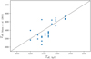Fig. C.1 Teff of Mann et al. (2015) vs Teff,SpT. The dotted line shows the 1:1 relation.

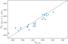Fig. C.2 Teff of Mann et al. (2015) vs $T_{\text{eff,}{ℳ}_{★}}$. The dotted line shows the 1:1 relation.

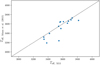Fig. C.3 Teff of Mann et al. (2015) vs Teff,M15. The dotted line shows the 1:1 relation.

Appendix D Tables

References

All Tables

All Figures

	Fig. 1 Model G2V spectra (yellow) and model M4V spectra (red). The flux scale of the G2V is displayed on the left, and the flux scale of the M4V is given on the right. The blue shaded area indicates the region of the Ca II H and K lines.
In the text

	Fig. 2 Ca II K line of an M1.5 star. Left: spectrum of a single HARPS observation. Right: template spectrum consisting of 47 coadded spectra of the same star.
In the text

	Fig. 3 High S/N template spectrum of an early-M dwarf normalized to a PHOENIX atmosphere model. The solid red line is the high S/N template spectrum, while the dashed black line is the PHOENIX model atmosphere. The blue shaded region shows the chromospheric emission. The dotted lines indicate the 1.09 Å FWHM triangular bandpass used to integrate the Ca II H and K lines.
In the text

	Fig. 4 High S/N template spectrum of an M dwarf with Hα in absorption normalized to a PHOENIX atmosphere model. The solid red line is the high S/N template spectrum, while the dashed black line is the PHOENIX model atmosphere. The vertical dotted lines indicate a 5.0 Å integration region.
In the text

	Fig. 5 High S/N template spectrum of an active M dwarf with Hα in emission normalized to a PHOENIX atmosphere model. The solid red line is the high S/N template spectrum, while the dashed black line is the PHOENIX model atmosphere. The vertical dotted lines indicate the 5.0 Å integration region of Hα.
In the text

	Fig. 6 SAD17 of Astudillo-Defru et al. (2017) vs our work SBS18 (Boro Saikia et al. 2018). Top: entire range of the sample. Bottom: same sample with zoomed in axes. The dotted line shows the 1:1 relation.
In the text

Fig. 7 Effective temperature Teff of the stellar sample using different Teff determination methods, which are shown by different plot symbols. Top: effective temperature Teff as a function of absolute magnitude $M_{K_S}$ with metallicity [Fe/H] shown according to the color scale. Temperatures of the same star are connected with a solid vertical line. Bottom: difference of the methods used to obtain Teff in K.

In the text

Fig. 8 Fractional chromospheric Ca II H and K flux normalized to bolometric flux on a logarithmic scale, log ${R^{\prime }}_{\text{HK}}$, as a function of absolute magnitude $M_{K_S}$. For each star, log ${R^{\prime }}_{\text{HK}}$ is calculated with different Teff calibrations, each plotted with a different color. Vertical gray lines connect different measurements of the same star. Triangles indicate stars exhibiting Hα emission. Filled symbols indicate stars without known planetary systems, and open symbols indicate stars with known planetary systems.

In the text

Fig. 9 Fractional chromospheric Ha flux, ${{ℱ}^{\prime }}_{\text{Hα}}/{ℱ}_{\text{bol}}$, as a function of absolute magnitude $M_{K_S}$. Vertical gray lines connect different measurements of the same star. Triangles indicate stars exhibiting Hα emission. Filled symbols indicate stars without known planetary systems, and open symbols indicate stars with known planetary systems. Values >0 indicate that Hα is in emission, and values <0 indicate that Hα is in absorption. Values near 0 indicate filling-in of the line to the continuum.

In the text

Fig. 10 Fractional chromospheric Hα flux, ${{ℱ}^{\prime }}_{\text{Hα}}$, as a function of fractional chromospheric Ca II H and K flux, ${{ℱ}^{\prime }}_{\text{HK}}$ flux. Filled symbols indicate stars without known planetary systems, and open symbols indicate stars with known planetary systems. Values >0 indicate that Hα is in emission, and values <0 indicate that Hα is in absorption. Values near 0 indicate filling-in of the line to the continuum.

In the text

Fig. 11 Fractional chromospheric Hα flux, ${{ℱ}^{\prime }}_{\text{Hα}}$, as a function of fractional chromospheric Ca II H and K flux, ${{ℱ}^{\prime }}_{\text{HK}}$ flux, both on a logarithmic scale. Filled symbols indicate stars without known planetary systems, and open symbols indicate stars with known planetary systems. In this plot, only stars with Hα in emission (>0) are shown. A linear fit is shown with a dashed red line, and a 1:1 relation is plotted as a dotted gray line.

In the text

Fig. 12 Different log Ccf calibrations as a function of Teff. The approximate spectral type is shown on the top axis. Top: PHOENIX stellar atmosphere models with different [Fe/H] and log(ɡ), where [Fe/H] is indicated by color and log(ɡ) indicated by symbol. The solid red line indicates a fifth-order polynomial fit. Bottom: calibrations of log Ccf from other works where only the valid calibration region is plotted. Overplotted in red is the same fifth-order polynomial fit from the top panel.

In the text

Fig. 13 Different log RHK,phot as a function of Teff. The approximate spectral type is shown on the top axis. Top: PHOENIX stellar atmosphere models with different [Fe/H] and log(ɡ), where [Fe/H] is indicated by color and log(ɡ) indicated by symbol. The solid red line indicates a fifth-order polynomial fit. Bottom: calibrations of log RHK,phot from other works where only the valid calibration region is plotted. Overplotted in red is the same fifth-order polynomial fit from the top panel.

In the text

Fig. 14 Top: continuum flux normalized to bolometric flux of Ca II H and K, χ Ca II HK, as a function of Teff using PHOENIX stellar atmospheres with log(ɡ) = 5.0 and different metallicities. Values from West & Hawley (2008) are plotted in gray. Bottom: continuum flux normalized to bolometric flux of Hα, χHα, as a function of Teff using PHOENIX stellar atmospheres with log(ɡ) = 5.0 and different metallicities. Values from West & Hawley (2008) are plotted in gray.

In the text

	Fig. C.1 Teff of Mann et al. (2015) vs Teff,SpT. The dotted line shows the 1:1 relation.
In the text

	Fig. C.2 Teff of Mann et al. (2015) vs $T_{\text{eff,}{ℳ}_{★}}$. The dotted line shows the 1:1 relation.
In the text

	Fig. C.3 Teff of Mann et al. (2015) vs Teff,M15. The dotted line shows the 1:1 relation.
In the text

References

- Anglada-Escudé, G., & Butler, R.P. 2012, ApJS, 200, 15 [CrossRef] [Google Scholar]
- Anglada-Escudé, G., Arriagada, P., Tuomi, M., et al. 2014, MNRAS, 443, L89 [NASA ADS] [CrossRef] [Google Scholar]
- Anglada-Escudé, G., Amado, P.J., Barnes, J., et al. 2016, Nature, 536, 437 [CrossRef] [Google Scholar]
- Astudillo-Defru, N., Delfosse, X., Bonfils, X., et al. 2017, A&A, 600, A13 [NASA ADS] [CrossRef] [EDP Sciences] [Google Scholar]
- Baliunas, S.L., Donahue, R.A., Soon, W.H., et al. 1995, ApJ, 438, 269 [NASA ADS] [CrossRef] [Google Scholar]
- Barden, S.C. 1985, ApJ, 295, 162 [NASA ADS] [CrossRef] [Google Scholar]
- Berdinas, Z.M., Amado, P.J., & Anglada-Escude, G. 2015, in 18th Cambridge Workshop on Cool Stars, Stellar Systems, and the Sun, eds. G.T. van Belle, & H.C. Harris, 18, 723 [NASA ADS] [Google Scholar]
- Bonfils, X., Delfosse, X., Udry, S., et al. 2013, A&A, 549, A109 [NASA ADS] [CrossRef] [EDP Sciences] [Google Scholar]
- Boro Saikia, S., Marvin, C.J., Jeffers, S.V., et al. 2018, A&A, 616, A108 [NASA ADS] [CrossRef] [EDP Sciences] [Google Scholar]
- Boyajian, T.S., von Braun, K., van Belle, G., et al. 2012, ApJ, 757, 112 [NASA ADS] [CrossRef] [Google Scholar]
- Cincunegui, C., Díaz, R.F., & Mauas, P.J.D. 2007, A&A, 469, 309 [NASA ADS] [CrossRef] [EDP Sciences] [Google Scholar]
- Delfosse, X., Forveille, T., Ségransan, D., et al. 2000, A&A, 364, 217 [NASA ADS] [Google Scholar]
- Duncan, D.K., Vaughan, A.H., Wilson, O.C., et al. 1991, ApJS, 76, 383 [NASA ADS] [CrossRef] [Google Scholar]
- Golimowski, D.A., Henry, T.J., Krist, J.E., et al. 2004, AJ, 128, 1733 [NASA ADS] [CrossRef] [Google Scholar]
- Gomes da Silva, J., Santos, N.C., Bonfils, X., et al. 2011, A&A, 534, A30 [NASA ADS] [CrossRef] [EDP Sciences] [Google Scholar]
- Gray, D.F. 2005, The Observation and Analysis of Stellar Photospheres (Cambridge: Cambridge University Press) [CrossRef] [Google Scholar]
- Hall, J.C., Lockwood, G.W., & Skiff, B.A. 2007, AJ, 133, 862 [NASA ADS] [CrossRef] [Google Scholar]
- Hartmann, L., Soderblom, D.R., Noyes, R.W., Burnham, N., & Vaughan, A.H. 1984, ApJ, 276, 254 [NASA ADS] [CrossRef] [Google Scholar]
- Herbig, G.H. 1985, ApJ, 289, 269 [NASA ADS] [CrossRef] [Google Scholar]
- Husser, T.-O., Wende-von Berg, S., Dreizler, S., et al. 2013, A&A, 553, A6 [NASA ADS] [CrossRef] [EDP Sciences] [Google Scholar]
- Kenyon, S.J., & Hartmann, L. 1995, ApJS, 101, 117 [NASA ADS] [CrossRef] [Google Scholar]
- Maldonado, J., Affer, L., Micela, G., et al. 2015, A&A, 577, A132 [NASA ADS] [CrossRef] [EDP Sciences] [Google Scholar]
- Maldonado, J., Scandariato, G., Stelzer, B., et al. 2017, A&A, 598, A27 [NASA ADS] [CrossRef] [EDP Sciences] [Google Scholar]
- Mann, A.W., Feiden, G.A., Gaidos, E., Boyajian, T., & von Braun, K. 2015, ApJ, 804, 64 [CrossRef] [Google Scholar]
- Martínez-Arnáiz, R., López-Santiago, J., Crespo-Chacón, I., & Montes, D. 2011, MNRAS, 414, 2629 [CrossRef] [Google Scholar]
- Middelkoop, F. 1982, A&A, 107, 31 [NASA ADS] [Google Scholar]
- Mittag, M., Schmitt, J.H.M.M., & Schröder, K.-P. 2013, A&A, 549, A117 [NASA ADS] [CrossRef] [EDP Sciences] [Google Scholar]
- Montes, D., de Castro, E., Fernandez-Figueroa, M.J., & Cornide, M. 1995a, A&AS, 114, 287 [NASA ADS] [Google Scholar]
- Montes, D., Fernandez-Figueroa, M.J., de Castro, E., & Cornide, M. 1995b, A&A, 294, 165 [NASA ADS] [Google Scholar]
- Neves, V., Bonfils, X., Santos, N.C., et al. 2012, A&A, 538, A25 [NASA ADS] [CrossRef] [EDP Sciences] [Google Scholar]
- Neves, V., Bonfils, X., Santos, N.C., et al. 2014, A&A, 568, A121 [NASA ADS] [CrossRef] [EDP Sciences] [Google Scholar]
- Newton, E.R., Irwin, J., Charbonneau, D., et al. 2017, ApJ, 834, 85 [NASA ADS] [CrossRef] [Google Scholar]
- Noyes, R.W., Hartmann, L.W., Baliunas, S.L., Duncan, D.K., & Vaughan, A.H. 1984, ApJ, 279, 763 [NASA ADS] [CrossRef] [Google Scholar]
- Passegger, V.M., Wende-von Berg, S., & Reiners, A. 2016, A&A, 587, A19 [NASA ADS] [CrossRef] [EDP Sciences] [Google Scholar]
- Pepe, F., Mayor, M., Rupprecht, G., et al. 2002, The Messenger, 110, 9 [NASA ADS] [Google Scholar]
- Perdelwitz, V., Mittag, M., Tal-Or, L., et al. 2021, A&A, 652, A116 [NASA ADS] [CrossRef] [EDP Sciences] [Google Scholar]
- Pérez Martínez, M.I., Schröder, K.-P., & Hauschildt, P. 2014, MNRAS, 445, 270 [CrossRef] [Google Scholar]
- Rauscher, E., & Marcy, G.W. 2006, PASP, 118, 617 [NASA ADS] [CrossRef] [Google Scholar]
- Reiners, A., & Basri, G. 2007, ApJ, 656, 1121 [NASA ADS] [CrossRef] [Google Scholar]
- Reiners, A., & Mohanty, S. 2012, ApJ, 746, 43 [Google Scholar]
- Reiners, A., Shulyak, D., Käpylä, P.J., et al. 2022, A&A, 662, A41 [NASA ADS] [CrossRef] [EDP Sciences] [Google Scholar]
- Ribas, I., Bolmont, E., Selsis, F., et al. 2016, A&A, 596, A111 [NASA ADS] [CrossRef] [EDP Sciences] [Google Scholar]
- Rutten, R.G.M. 1984, A&A, 130, 353 [NASA ADS] [Google Scholar]
- Scandariato, G., Maldonado, J., Affer, L., et al. 2017, A&A, 598, A28 [NASA ADS] [CrossRef] [EDP Sciences] [Google Scholar]
- Shulyak, D., Seifahrt, A., Reiners, A., Kochukhov, O., & Piskunov, N. 2011, MNRAS, 418, 2548 [NASA ADS] [CrossRef] [Google Scholar]
- Suárez Mascareño, A., Rebolo, R., González Hernández, J.I., & Esposito, M. 2015, MNRAS, 452, 2745 [CrossRef] [Google Scholar]
- Suárez Mascareño, A., Rebolo, R., & González Hernández, J.I. 2016, A&A, 595, A12 [NASA ADS] [CrossRef] [EDP Sciences] [Google Scholar]
- Vaughan, A.H., & Preston, G.W. 1980, PASP, 92, 385 [CrossRef] [Google Scholar]
- Walkowicz, L.M., & Hawley, S.L. 2009, AJ, 137, 3297 [NASA ADS] [CrossRef] [Google Scholar]
- Walkowicz, L.M., Hawley, S.L., & West, A.A. 2004, PASP, 116, 1105 [CrossRef] [Google Scholar]
- Wenger, M., Ochsenbein, F., Egret, D., et al. 2000, A&AS, 143, 9 [NASA ADS] [CrossRef] [EDP Sciences] [Google Scholar]
- West, A.A., & Hawley, S.L. 2008, PASP, 120, 1161 [CrossRef] [Google Scholar]
ESO IDs 082.C-0718 and 183.C-0437.
ESO ID 191.C-0505.