| Issue |
A&A
Volume 536, December 2011
|
|
|---|---|---|
| Article Number | A38 | |
| Number of page(s) | 11 | |
| Section | Interstellar and circumstellar matter | |
| DOI | https://doi.org/10.1051/0004-6361/201117791 | |
| Published online | 05 December 2011 | |
Unveiling the gas kinematics at 10 AU scales in high-mass star-forming regions
Milliarcsecond structure of 6.7 GHz methanol masers
1
INAF – Osservatorio Astrofisico di Arcetri, Largo E. Fermi 5, 50125 Firenze, Italy
e-mail: This email address is being protected from spambots. You need JavaScript enabled to view it.
2
Max-Planck-Institut für Radioastronomie, Auf dem Hügel 69, 53121 Bonn, Germany
e-mail: This email address is being protected from spambots. You need JavaScript enabled to view it.
3
European Southern Observatory, Karl-Schwarzschild-Strasse 2, 85748 Garching bei München, Germany
e-mail: This email address is being protected from spambots. You need JavaScript enabled to view it.
Received: 29 July 2011
Accepted: 12 September 2011
Abstract
Context. High-mass stars play a prominent role in Galactic evolution, but their formation mechanism is still poorly understood. This lack of knowledge reflects the observational limitations of present instruments, whose angular resolution (at the typical distances of massive protostars) precludes probing circumstellar gas on scales of 1–100 AU, relevant for a detailed investigation of accretion structures and launch/collimation mechanims of outflows in high-mass star formation.
Aims. This work presents a study of the milliarcsecond structure of the 6.7 GHz methanol masers at high-velocity resolution (0.09 km s-1) in four high-mass star-forming regions: G16.59−0.05, G23.01−0.41, IRAS 20126 + 4104, and AFGL 5142.
Methods. We studied these sources by means of multi-epoch VLBI observations in the 22 GHz water and 6.7 GHz methanol masers, to determine the 3-D gas kinematics within a few thousand AU from the (proto)star. Our results demonstrate the ability of maser emission to trace kinematic structures close to the (proto)star, revealing the presence of fast wide-angle and/or collimated outflows (traced by the H2O masers), and of rotation and infall (indicated by the CH3OH masers). The present work exploits the 6.7 GHz maser data collected so far to investigate the milliarcsecond structure of this maser emission at high-velocity resolution.
Results. Most of the detected 6.7 GHz maser features present an ordered (linear, or arc-like) distribution of maser spots on the plane of the sky, together with a regular variation in the spot LSR velocity (VLSR) with position. Typical values for the amplitude of the VLSR gradients (defined in terms of the derivative of the spot VLSR with position) are found to be 0.1–0.2 km s-1 mas-1. In each of the four target sources, the orientation and the amplitude of most of the feature VLSR gradients remain remarkably stable in time, on timescales of (at least) several years. We also find that the data are consistent with having the VLSR gradients and proper motion vectors in the same direction on the sky, considered the measurement uncertainties. In three (G16.59 − 0.05, G23.01 − 0.41, and IRAS 20126 + 4104) of the four sources under examination, feature gradients with the best determined (sky-projected) orientation divide into two groups directed approximately perpendicular to each other.
Conclusions. The time persistency, the ordered angular and spatial distribution, and the orientation generally similar to the proper motions, altogether suggest a kinematical interpretation for the origin of the 6.7 GHz maser VLSR gradients. This work shows that the organized motions (outflow, infall, and rotation) revealed by the (22 GHz water and 6.7 GHz methanol) masers on large scales (~100–1000 AU) also persist to very small (~10 AU) scales. In this context, the present study demonstrates the potentiality of the mas-scale 6.7 GHz maser gradients as a unique tool for investigating the gas kinematics on the smallest accessible scales in proximity to massive (proto)stars.
Key words: masers / techniques: high angular resolution / techniques: spectroscopic / ISM: kinematics and dynamics / ISM: structure / stars: formation
© ESO, 2011
1. Introduction
Intense maser transitions of the OH (at 1.6 and 6.0 GHz), CH3OH (at 6.7 and 12 GHz), H2O (at 22 GHz), and SiO (at 43 GHz) molecules, are observed towards massive star-forming regions. The elevate brightness temperature ( ≥ 107 K) of the maser emissions permits us to observe them with the Very Long Baseline Interferometry (VLBI) technique, achieving both very high angular (1–10 mas) and velocity (0.1 km s-1) resolution. Maser VLBI observations are the unique mean by which one can explore the gas kinematics close (within tens or hundreds of AU) to the forming high-mass (proto)star (e.g., Goddi et al. 2005; Sanna et al. 2010a,b; Matthews et al. 2010; Moscadelli et al. 2011), and they have also been successfully used to infer the properties of the magnetic field inside molecular cores (Fish & Reid 2006).
VLBI maser observations are useful for testing the present theories of massive star formation. To overcome the radiation pressure exerted by the already ignited star and still enable mass accretion, most models point to the essential role that accretion disks and jets should play. The former focus the ram pressure of the accreting matter across the disk plane, and the latter channel stellar photons along the jet axis and lower the radiation pressure across the equatorial plane. However, so far, interferometric observations of thermal continuum and line emissions towards massive star-forming regions have only identified a handful of disk candidates in association with high-mass stars (see e.g., Cesaroni et al. 2006). In particular, no circumstellar disks have been detected around early O-type stars, where only huge, massive, rotating structures are seen, whose lifetimes appear to be less than the corresponding rotation periods (see e.g., Beltrán et al. 2011). One reason that could explain the difficulty detecting disks in massive star-forming regions (with typical distances of a few kpc) is that the angular resolution ( ≥ 1″) achieved by present millimeter interferometers could not suffice to resolve disks if their size, as models predict, is comparable to or less than a few thousand AU. On the contrary, supposing one can observe a masing transition from the disk gas, the angular resolution achievable with maser VLBI observations is high enough to accurately measure the rotation curve of the accretion disk.
For a decade we have been studying a sample of ten candidate high-mass (proto)stars by means of VLBI observations of H2O 22 GHz, CH3OH 6.7 GHz, and OH 1.6 GHz masers associated with the (proto)stellar environment. The H2O and CH3OH masers are observed at several epochs to derive the maser proper motions, which, knowing the distance to the maser source, can be translated into the sky-projected components of the maser velocity. Combining this information with the line-of-sight velocity components, which are derived from the maser LSR velocity (VLSR) and the knowledge of the (proto)star systemic VLSR, a full 3-D picture of the motion of the masing gas can be obtained. So far, data for four sources have been analyzed: G16.59 − 0.05 (Sanna et al. 2010a, hereafter SMC1), G23.01 − 0.41 (Sanna et al. 2010b, hereafter SMC2), IRAS 20126 + 4104 (Moscadelli et al. 2011, hereafter MCR), and AFGL 5142 (Goddi et al. 2007, 2011, hereafter GMS1 and GMS2, respectively). These results demonstrate the ability of maser emission to trace kinematic structures close to the (proto)star, revealing fast wide-angle and/or collimated outflows (traced by the H2O masers) and rotation and infall (indicated by the CH3OH masers).
The present work exploits the 6.7 GHz maser data collected so far to investigate the milliarcsecond structure of this maser emission at high-velocity resolution. Since the velocity resolution of the 6.7 GHz maser dataset (0.09 km s-1) is high enough to resolve the maser emission linewidth (with typical FWHM of 0.3 km s-1), by mapping each velocity channel across the maser linewidth, one can investigate how the spatial structure of the emission changes with the velocity. A similar study has been previously performed for the intense 1.6 GHz (Fish et al. 2006) and 6.0 GHz (Fish & Sjouwerman 2007) OH and 12 GHz CH3OH (Moscadelli et al. 2003) masers in the UC Hii region W3(OH). These observations have revealed that it is quite common to observe a regular variation (along a line or an arc) in the maser peak position with the VLSR. In W3(OH), 1.6 and 6.0 GHz OH masers and 12 GHz CH3OH masers are found to have similar amplitudes of the VLSR gradients (calculated by dividing the maser VLSR linewidth by the path length over which the maser peak position shifts on the plane of the sky), varying in the range 0.01–1 km s-1 AU-1.
This paper extends the study of the milliarcsecond structure of the maser emission at high-velocity resolution to the 6.7 GHz CH3OH masers, presenting results in four distinct massive star-forming regions: G16.59 − 0.05, G23.01 − 0.41, IRAS 20126 + 4104, and AFGL 5142. Section 2 summarizes the main observational parameters of the EVN 6.7 GHz observations towards these sources. Section 3 describes the basic characteristics of the milliarcsecond, velocity structure of the 6.7 GHz masers, making use of our multi-epoch observations to also examine the time variation. Section 4 compares the directions on the sky plane of the maser VLSR gradients and proper motion vectors. Section 5 compares the results obtained among the four sources and discusses a possible interpretation of the time-persistent velocity gradients inside most of the 6.7 GHz maser cloudlets.
2. Summary of CH3OH 6.7 GHz maser EVN observations
Using the European VLBI Network (EVN)1, we observed the sources G16.59 − 0.05, G23.01 − 0.41, IRAS 20126 + 4104, and AFGL 5142 in the 51–60 A+ CH3OH transition (rest frequency 6.668519 GHz), at three different epochs, over the years 2004–2009. Table 1 lists the EVN observing epochs for each of the four sources, and gives the bibliographic reference of the articles where the results of these observations have been published. We refer the reader to these articles both for a full description of the EVN observing setup and for a discussion of the 3-D gas kinematics close to the massive (proto)star as traced by the H2O 22 GHz and CH3OH 6.7 GHz masers.
To determine the 6.7 GHz maser absolute positions and velocities, the EVN observations were performed in phase-referencing mode, by fast switching between the maser source and one strong, nearby calibrator. For each of the four maser targets, the selected phase-reference calibrator (belonging to the list of sources defining the International Celestial Reference Frame, ICRF) has an angular separation on the sky from the maser less than 3°. In each of the four targets, the absolute position of the 6.7 GHz masers is derived with an accuracy of a few milliarcseconds.
The antennae involved in the observations were Medicina, Cambridge, Jodrell, Onsala, Effelsberg, Noto, Westerbork, Torun, Darnhall, and Hartebeesthoek. Because of technical problems, the Darnhall telescope replaced the Jodrell antenna in the first epoch (November 2004) of the IRAS 20126 + 4104 and AFGL 5142 EVN observations. The Hartebeesthoek antenna took part in the observations only for the first two epochs of the low-DEC sources G16.59 − 0.05 and G23.01 − 0.41. In the third epoch, since the maser emission would be heavily resolved on the longest baselines involving the Hartebeesthoek antenna, it was replaced with the Onsala telescope. All the EVN runs had a similar observing setup, providing the same velocity resolution of 0.09 km s-1, and a similar sensitivity, corresponding to a thermal rms noise level on the channel maps of ~ 10 mJy beam-1.
CH3OH 6.7 GHz EVN observations.
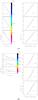 |
Fig. 1 Examples of two 6.7 GHz maser features with ordered spatial and VLSR distribution. a) The upper, middle, and lower panels refer to measurements at the first, second, and third observing epochs, respectively. Left panels: spot spatial distribution. Triangles, squares, and pentagons indicate the spot positions on the plane of the sky at the first, second, and third epochs, respectively, with symbol size varying logarithmically with the spot intensity. The symbol color indicates the spot VLSR, with the color-velocity conversion code given in the wedge on the right side of the three panels. At each epoch, the positions of the spots are relative to that of the epoch’s most intense spot. In each of the three panels, the continuous line shows the (minimum χ2) linear fit to the spot positions, defining the direction of the major axis of the spot distribution. The lower left corner of each panel reports the value of the linear correlation coefficient, rs. Right panels: spot VLSR-position distribution. In each of the three panels, empty circles show the plot of spot VLSR versus the position offset along the major axis of the spot distribution. Position offsets are taken as positive if increasing towards the east. Circle size varies logarithmically with the spot intensity. The continuous lines show the (minimum χ2) linear fit to the circle distribution. The lower right corner of each panel reports the value of the linear correlation coefficient, rv. b) Same as for a) for another feature of our sample. |
As indicated in Table 1, the EVN observations achieved comparable angular resolutions towards the four target sources, with some larger beams for the two sources at low DEC, because of the degraded uv-coverage. Isolated 6.7 GHz maser emission centers on a single-channel map (named “spots”) are generally unresolved or slightly resolved with the EVN. By fitting a two-dimensional elliptical Gaussian to the spot intensity distribution, the accuracy in the relative positions of maser spots, δθ, can be calculated through the formula δθ = 0.5 FWHM/SNR, where FWHM is the fitted spot size (about the FWHM beam size for a compact source) and SNR is the ratio of the spot intensity with the image rms noise. Since most of the detected spots have intensities ≥ 1 Jy and SNR ≥ 100, their relative positions are known with an accuracy better than 0.1 mas.
3. Results
In the following we use the term “spot” to point to a compact emission center on a single-channel map and the term “feature” to refer to a collection of spots emitting in contiguous channels at approximately the same position on the sky (within the beam FWHM). In our view, a maser feature corresponds to a distinct, masing cloud of gas, whose spatial and velocity structure is the subject of our analysis.
3.1. 6.7 GHz maser internal VLSR gradients
Figure 1 presents the spatial distribution and the change in VLSR with position of the spots belonging to two 6.7 GHz maser features, selected to be representative of the ordered VLSR gradients commonly found inside the 6.7 GHz masers. The examples presented in Fig. 1 are two intense, persistent features from the source G23.01 − 0.41. At each of the three observing epochs, spots from a given feature distribute in space close to a line and show a regular variation in VLSR versus the position measured along the feature major axis (see also Fig. 6 in SMC1). In the following discussion, we use rs and rv to indicate the correlation coefficients of the linear fit to the spot positions on the sky plane and to the VLSR variation with position (measured along the major axis of the spot distribution), respectively. For the maser feature in Fig. 1a, the linear fits of both the sky-projected spot distribution and the variation in VLSR with position always have a correlation coefficient equal to 1. For the feature in Fig. 1b, the spatial and velocity distribution of the spots is less ordered, with correlation coefficients of the linear fits in the range 0.4–1.0.
The linear fits presented in Fig. 1 were performed for each feature (of the four maser sources) with three or more spots, thereby deriving the following quantities: the PA of the feature (major axis) orientation on the sky plane, Ps, with the degree of linear correlation of the spot distribution on the sky plane measured by rs; and the amplitude of the VLSR gradient with position, Γ (in units of [km s-1 mas-1]), with the degree of linear correlation of VLSR with position (measured along the feature major axis) given by rv. With the adopted convention, that position’s offsets along the feature major axis are taken as positive if increasing to east, VLSR increasing to east (west) results into positive (negative) velocity gradients. Then, the PA of the feature orientation, Ps, varies in the range 0°–180° for positive gradients, and in the range 180°–360° for negative gradients. The measurement errors of both the spot positions (≤0.1 mas) and VLSR (≤0.09 km s-1) are small enough with respect to the typical extension of the feature spot distribution (from a few mas to 10 mas) and feature emission width (0.5–1 km s-1) not to affect the precision with which the orientation and the amplitude of the feature gradient can be determined.
The examples shown in Fig. 1 are not rare cases among the 6.7 GHz maser features. For each of the four target sources, Fig. 2 presents the histograms of the correlation coefficients rs and rv of the linear fits performed on all the features with three or more spots. A large fraction (60–80%) of the correlation coefficients showing values higher than 0.6, indicates that, in each source, a vast majority of maser features has a spatial structure primarily elongated in one direction, and also presents (at least) a hint of a regular variation in VLSR along this direction. Besides, more than half of the features present a well-defined linear structure with quite a regular change in VLSR with position, since more than half of the derived values of rs and rv are higher than 0.8. We note that, in each source, the distribution of rv is more peaked at higher values than that of rs. That means that there are features showing a good correlation of VLSR with position measured along the major axis of elongation, even if their structure is only marginally elongated. Figure 1b illustrates this case for a representative feature.
Figure 3 presents the histograms of the amplitude of the VLSR gradients for the observed maser sources. To produce the histograms and calculate the average and standard deviation of the distributions, we selected only those features that presented at least some evidence of being elongated (rs ≥ 0.6) and that showed a hint of a regular VLSR variation with position (rv ≥ 0.6). The average amplitude of the VLSR gradients for the sources G23.01 − 0.41 and G16.59 − 0.05 ( ≈ 0.2 km s-1 mas-1) is about twice the value derived for the sources IRAS 20126 + 4104 and AFGL 5142 ( ≈ 0.1 km s-1 mas-1).
The knowledge of an accurate value of the source distance would allow us to convert the amplitude of VLSR gradients from units of [km s-1 mas-1] to units of [km s-1 AU-1] and to compare the gradient amplitudes of different sources. Recently, the distance to two of the sources has been precisely determined by measuring the parallax of the associated, strong methanol, and water masers: IRAS 20126 + 4104 is at a distance of 1.64 ± 0.05 kpc (MCR), and G23.01 − 0.41 is at 4.59 ± 0.4 kpc (Brunthaler et al. 2009). After converting to units of [km s-1 AU-1], one finds that the distribution of gradient amplitudes in IRAS 20126 + 4104 (0.07 ± 0.04 km s-1 AU-1) overlaps with the one in G23.01 − 0.41 (0.05 ± 0.05 km s-1 AU-1), although the (proto)stars associated to the CH3OH masers in IRAS 20126 + 4104 and G23.01 − 0.41 have very different luminosities and masses (MCR, SMC2). That lets us argue that the VLSR gradients internal to the 6.7 GHz masers might have a common origin in the two sources, resulting in comparable values of gradient amplitudes. Also for the sources G16.59 − 0.05 and AFGL 5142 (using the more uncertain distance of 4.4 kpc and 1.8 kpc, respectively), the values of the gradient amplitude, in units of [km s-1 AU-1], are consistent with those of IRAS 20126 + 4104 and G23.01 − 0.41.
3.2. Time persistency of VLSR gradients
As defined in Sect. 3.1, VLSR gradients are vector quantities, oriented on the sky plane at PA = Ps and with amplitude Γ. For the two features presented in Fig. 1, the direction on the sky plane and the amplitude of the VLSR gradient appear to be fairly constant over the three observing epochs. To investigate the variation in VLSR gradients with time, we selected features persistent over two or three epochs and calculated the standard deviation of the direction (ΔPs) and amplitude (ΔΓ) of the feature VLSR gradient at different epochs. The (time-average) mean gradient is calculated by taking the mean values of the gradient components projected along the east and the north directions. For a persistent feature, the change in time of the gradient amplitude is measured by the “fractional time variation” (ΔΓ/Γ), defined as the ratio of the standard deviation, ΔΓ, and the mean of the values of the feature gradient amplitude, Γ, at different epochs.
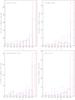 |
Fig. 2 Histograms of the linear correlation coefficients rs and rv. Each panel presents the histograms of rs (blue dotted line) and rv (red dashed line), for one of the four maser sources, indicated in the upper left corner of the panel. The bin size is 0.1. |
Figure 4 presents the histograms of ΔPs and ΔΓ/Γ for each of the four maser sources. In each source, on a timescale of several years, the amplitude of the VLSR gradient for most of the persistent features changes less than 20–40%, and the variation in the gradient orientation is generally less than 20°. Measurement errors can contribute to enlarge the calculated spreads in time, so that the effective time variation could be even smaller than what is shown in Fig. 4. Therefore, we can conclude that most of the 6.7 GHz maser internal VLSR gradients appear to be remarkably stable in time on a timescale of (at least) several years.
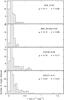 |
Fig. 3 Histograms of the amplitude of the VLSR gradient, Γ. Each panel plots data of a single maser source, indicated in the upper right corner of the panel. The bin size of all the histograms is 0.05 km s-1 mas-1. Each panel (below the source name) also reports the arithmetic average, μ, and the standard deviation, σ, of the gradient amplitude, in units of [km s-1 mas-1]. |
3.3. Ordered spatial and angular distribution of VLSR gradient directions
For each of the four maser sources, Fig. 5 shows the distribution on the plane of the sky of the directions of VLSR gradients and the histogram of the PA of gradient directions. To produce these plots, we neglected the sign of the VLSR gradient, and the PA of negative gradients (180° ≤ Ps ≤ 360°) was folded into the range 0°–180°.
Looking at the histograms of the gradient PA, it is evident that, in each of the four sources, the directions of feature gradients do not distribute uniformly, but tend to concentrate into specific PA ranges. For the sources G23.01−0.41, G16.59−0.05, and IRAS 20126+4104, the PA distribution presents two broad, but clearly distinct peaks at the angles 40° ± 20° and 140° ± 20°. For the source AFGL 5142, only a single, broad peak, over the angles 90° ± 30°, is clearly visible. For the sources G23.01−0.41, G16.59−0.05, and IRAS 20126+4104, with a larger number of detected maser features and better statistics, the peaks in the distribution of gradient PA become narrower when selecting gradients with increasingly better measured directions (i.e. corresponding to linear fits with increasingly higher values of the correlation coefficient, rs). That reinforces the impression that the two-peak distribution has a physical meaning, and it does not result from a bias in our data analysis.
The plots of the spatial distribution of the VLSR gradient directions illustrate that, in the sources G23.01 − 0.41, G16.59 − 0.05, and IRAS 20126 + 4104, the two groups of features with gradients approximately perpendicular to each other, are not confined in two different regions of the sky, but are spread over a similar area and are observed to almost overlap (with separation of only ≈ 10 mas) along some lines-of-sight. In these three maser sources, the two groups of gradients also have a similar spatial distribution of VLSR. The case of the source AFGL 5142 may be different. In this source, the more red-shifted features, confined to the south and southeast of the whole maser distribution, have VLSR gradients directed close to east-west (PA ≈ 90°), whereas most of the “yellow” features, placed to the north and northwest, show gradients directed close to north-south (PA ≈ 0° or 180°). For this source, the poor statistics of well-measured gradient orientations very likely prevents us from clearly detecting a second peak in the distribution of gradient PA close to 0° and/or 180°. In any case, in AFGL 5142, differently from the other three sources, the direction of the maser VLSR gradient appears to be correlated with the feature position.
Section 5 discusses the peculiarities observed in the spatial and angular distribution of the 6.7 GHz maser VLSR gradients, and proposes a simple kinematical interpretation.
4. Comparison with 6.7 GHz maser proper motions
The time persistency of most of the 6.7 GHz maser VLSR gradients on timescales of (at least) several years, and the regular (spatial and angular) distribution of the gradient directions observed towards all the four maser targets suggests that the maser internal gradients might reflect the ordered gas motions observed over the whole maser region (size of ~100–1000 AU) on small (linear) scales (~10 AU). In all sources but G16.59 − 0.05, our 22 GHz water maser observations show a fast wide-angle wind and/or a collimated jet emerging from the same (proto)star exciting the methanol masers. Over the whole region, the 6.7 GHz masers present a rather ordered 3-D kinematics, suggesting either rotation (in G16.59 − 0.05), a combination of rotation plus expansion (G23.01 − 0.41 and IRAS 20126 + 4104), or infall (AFGL 5142).
If the VLSR gradients internal to the 6.7 GHz masers reflect ordered, large-scale gas motions, one would expect them to be related to the gas velocities. For instance, should the VLSR gradients be produced in either a rotating structure or a Hubble outflow, one would expect the directions of the feature gradient and proper motion to project at a close angle on the sky. Figure 6 presents the source-average distribution of the angle between the direction of the VLSR gradient of a maser feature and its proper motion vector. The 6.7 GHz maser proper motions are read from Table 3 of SMC1 for G16.59 − 0.05, from Table 4 of SMC2 for G23.01 − 0.41, from Table 1 of MCR for IRAS 20126 + 4104, and from GMS2 for AFGL 5142. The acute angle between the feature gradient and proper motion directions on the sky plane is used to measure the angular separation. To produce the plot in Fig. 6, feature gradients with loosely defined directions (i.e. with rs ≤ 0.5 and rv ≤ 0.5) were discarded, and, for persistent features, the mean gradient averaged over the three epochs was calculated. Features that have both the VLSR gradient and the proper motion reliably measured, are a few tens for the sources G23.01 − 0.41 (36) and AFGL 5142 (20), but significantly less for G16.59 − 0.05 (8) and IRAS 20126 + 4104 (7). To increase the statistics, we calculated the distribution of the fractional number of features for each source (dividing the number of features of a histogram bin by the total number of features), and then averaged over the four sources.
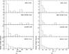 |
Fig. 4 Time variation in VLSR gradient PA and amplitude. a) Each of the four panels refers to the maser source indicated in the upper right corner of the panel, and presents the histogram of the standard deviation (ΔPs) of the values of the gradient PA, at different epochs, for features persisting over two or three observing epochs. The bin size of all the histograms is 10°. b) Each of the four panels refers to the maser source indicated in the upper right corner of the panel, and presents the histogram of the fractional time variation (ΔΓ/Γ) in the gradient amplitude, for features persisting over two or three observing epochs. The bin size of all the histograms is 0.2. |
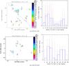 |
Fig. 5 The panels in each row present the spatial distribution and the histogram of the VLSR gradient directions for the maser source indicated below the panels. Left panel: spatial distribution of the VLSR gradient directions. Colored dots report the position of the maser features detected over the three observing epochs, with colors indicating the feature VLSR. The velocity-color conversion code is shown in the wedge on the right side of the panel, with green denoting the systemic VLSR of the maser source. Colored segments associated to maser features give the direction of the feature VLSR gradient (with PA varying in the range 0°–180°), with different colors to distinguish the observing epoch: red, green, and blue, for the first, second, and third epochs, respectively. The segment length is proportional to the value of the correlation coefficient, rs, of the linear fit to the spot positions, from which the gradient direction is derived. The plot reports only the feature gradients with better defined directions, corresponding to more linear spot distributions and higher values of the correlation coefficient, rs: rs > 0.9 for G23.01 − 0.41, and rs > 0.8 for G16.59−0.05. For the sources G16.59−0.05 and G23.01 − 0.41, feature positions are relative to the maser’s “center of motion”, as defined in SMC1 and SMC2, respectively. In the plot of G23.01−0.41, the dashed arrow indicates the direction of the collimated jet traced close to the (proto)star by the 22 GHz water masers (SMC2). Right panel: histograms of the PA of the feature gradient directions. Dotted black, dashed red, and continuous blue lines show the histograms of the gradient PA for features with increasingly better linear structure, corresponding to values of the correlation coefficient rs > 0, rs > 0.5, and rs > 0.9, respectively. The histogram bin size is 15° for the source G23.01−0.41, and 20° for the source G16.59−0.05. |
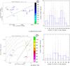 |
Fig. 5 continued. The panels in each row present the spatial distribution and the histogram of the VLSR gradient directions for the maser source indicated below the panels. Left panel: spatial distribution of the VLSR gradient directions. Colored dots and colored segments have the same meaning as in Figs. 5a and b. For the source IRAS 20126 + 4104, absolute maser positions are reported, relative to the observing epoch 2004 November 6 (MCR, Fig. 2). In the source AFGL 5142, feature positions are relative to the peak of the VLA 1.3 cm continuum observed toward the 6.7 GHz masers (Goddi et al. 2007, see Fig. 2), whose contour map is shown by a dotted line. In both the plots of IRAS 20126 + 4104 and AFGL 5142, the dashed line gives the direction of the collimated jet traced close to the (proto)star by the 22 GHz water masers. The plot reports only the feature gradients with better defined directions, corresponding to more linear spot distributions and higher values of the correlation coefficient, rs: rs > 0.8 for IRAS 20126 + 4104, and rs > 0.6 for AFGL 5142. Right panel: histograms of the PA of the feature gradient directions. Dotted black, dashed red, and continuous blue lines have the same meaning as in Figs. 5a and 5b. The histogram bin size is 15° for the source IRAS 20126 + 4104, and 20° for the source AFGL 5142. |
Figure 6 provides some evidence that the VLSR gradients tend to be oriented at relatively small angles ( ≤ 40°) from the direction of the maser proper motions. The actual distribution might be significantly more peaked at small angles than observed, since the uncertainty in the measurements of the gradient and proper motion orientations can be large ( ≥ 20°), and can contribute significantly to broaden the peak. The basic characteristics of the source-average plot of Fig. 6 do not result from one source’s distribution dominating the other ones, but, conversely, in all four sources there is a similar tendency towards small angular separations between the maser gradients and proper motions. Therefore we can conclude that in each of the observed sources, the data are consistent with having the VLSR gradients and proper motion vectors in the same direction on the sky, considered the measurement uncertainties.
Fish et al. (2006), studying the 1.6 GHz OH masers towards the W3(OH) UC Hii region, did not note any correlation between the orientation of the VLSR gradients and the proper motions of the OH masers (measured by Bloemhof et al. 1992). Over the whole extent of the UC Hii region ( ≈ 3000 AU in size), Fish et al. (2006) and Fish & Sjouwerman (2007) did not find any large-scale organization in the distribution of the OH VLSR gradients, and then suggest that the observed gradients should trace local phenomena, which are possibly associated to AU-scale turbulent fluctuations in the sky-projected velocity field. However, the environment traced by the 6.7 GHz masers in each of our target sources appears to be different from that of an UC Hii region. The typical 6.7 GHz maser velocities (5–10 km s-1) are significantly higher than those of the OH masers in W3(OH) (a few km s-1). Whereas in W3(OH) and in other sources as well (G23.01 − 0.41; see SMC2), the OH masers appear to mark gas at greater distance ( ≥ 103–104 AU) from the (proto)star and to trace the slow expansion of the UC Hii region, the 6.7 GHz masers are more likely associated with gas accreting, rotating, and outflowing, in the proximity (within hundreds of AU) to the (proto)star. Differently from the OH, we believe that the measured gradients of CH3OH masers trace gas kinematics on AU-scales, as discussed in detail in the next section.
5. Nature of the 6.7 GHz maser VLSR gradients
In the following, we discuss the hypothesis that the 6.7 GHz maser VLSR gradients trace, on very small scale ( ≲ 10 AU), the bulk-ordered motion measured on large scales from maser kinematics: outflow or infall (Sect. 5.1) and rotation (Sect. 5.2) in high-mass (proto)stars.
5.1. Do methanol maser VLSR gradients trace outflow/infall?
We consider first the case that the 6.7 GHz maser VLSR gradients are associated with the large-scale outflows traced by the water masers in the sources G23.01 − 0.41, IRAS 20126 + 4104 and AFGL 5142.
In the source IRAS 20126 + 4104, the 3-D velocity field of the 22 GHz water masers has been successfully reproduced with a model of a conical, Hubble flow, with maser velocities increasing linearly with the distance from the star. Assuming that the water maser velocity distribution can also be described in terms of an Hubble flow in the other sources, from the measured 3-D velocities it is possible to derive a typical velocity gradient in the outflowing gas. Considering that the observed water masers generally move close to the plane of the sky, one has to divide the maximum observed value of transverse velocities by the sky-projected semi-length of the outflow. This calculation gives a gradient of 0.2 km s-1 mas-1 and 0.15 km s-1 mas-1 for the jets observed in the sources AFGL 5142 and IRAS 20126 + 4104, respectively. For the source G23.01 − 0.41, we obtain a gradient of 0.5 km s-1 mas-1 for the fast and compact wide-angle wind located close to the (proto)star and a much lower value of 0.06 km s-1 mas-1 for the collimated jet traced by two groups of water masers at a greater distance from the (proto)star. In each of the three sources, the gradient in the outflow velocities derived from the water masers is an upper limit to the average value of the 6.7 GHz maser VLSR gradients (see Fig. 3). That is consistent with the fact that 6.7 GHz masers are found to move much more slowly than water masers do. One possible interpretation is that water masers trace fast, shocked gas closer to the jet axis, while methanol masers might originate in relatively slow-moving material, entrained in the outflow at a larger distance from the jet axis. Looking at specific cases, in the source IRAS 20126 + 4104 MCR show that the entraining process takes place for a group of 6.7 GHz features with proper motions directed close to the jet direction, while for the source AFGL 5142 we propose that the 6.7 GHz maser 3-D velocities trace infall rather than outflow. Regardless of the specific source case, this simple discussion shows that, in each of the three sources where an outflow or infall is detected, the gas moves fast enough to be able to account for the VLSR gradients internal to the 6.7 GHz masers.
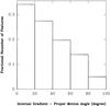 |
Fig. 6 Histogram of the distribution of the angle between the direction of the VLSR gradient of a maser feature and its proper motion vector. The histogram bin size is 20°. The histogram reports the fractional number of maser features averaged over the four target sources. |
Figure 5 shows that the directions of the VLSR gradients in three sources tend to cluster in two PA ranges (separated by about 90°–100°), while a single peak in the distribution of gradient PA is evident for the source AFGL 5142. For the three sources with an observed water maser jet, the orientation of the jet axis is reported in the plot of the spatial distribution of gradient directions. It is interesting to note that, for both sources G23.01−0.41 and IRAS 20126 + 4104, the PA of the jet axis (about 50° and 115° for the first and second sources, respectively) is close to one of the two peaks in the distribution of gradient PA. We consider that, while the direction of the jet axis is the one along which VLSR gradients associated with the outflow should project, the direction perpendicular to the jet should be the preferred orientation of gradients due to (almost edge-on) rotation about the jet. This qualitative argument can simply explain the presence of the two peaks in the distribution of gradient PA for the sources G23.01 − 0.41 and IRAS 20126 + 4104, and lends further support to the idea of a correlation between the small-scale VLSR gradients inside the 6.7 GHz maser features and the ordered gas motions observed over the whole maser region.
5.2. Do methanol maser VLSR gradients trace rotation?
One of the simplest interpretations of a regular change in VLSR with position across the plane of the sky is in terms of rotation. If the spots of a 6.7 GHz maser feature traced a portion of an annulus of a rotating sphere of gas, seen almost edge-on, that could explain the (sky-projected) linear distribution of spots and also the linear variation in VLSR with (sky-projected) spot positions. Assuming that the rotation is gravitationally supported, one can easily derive a relation between the average gas (mass) density,  , and the measured gradient amplitude, Γ:
 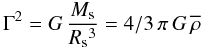 (1)where G is the gravitational constant, and Ms and Rs are the mass and the radius of the sphere, respectively. Using an average value of Γ = 0.05 km s-1 AU-1 (as derived above for the sources IRAS 20126 + 4104 and G23.01 − 0.41), one finds
  g cm-3, corresponding to a number density of hydrogen molecules nH2 = 1011 cm-3. Using this average density, indicating with R10 the radius of the maser annulus in units of 10 AU, the mass of the gas sphere inside the annulus radius is
 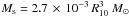 .
.
The obtained value of  and the expression for Ms can be used to further constrain the properties of the putative rotation traced by the 6.7 GHz maser VLSR gradients. Excitation models of the 6.7 GHz methanol masers (Cragg et al. 2005) predict that this maser emission should be quenched for nH2 ≥ 109 cm-3. Since this value is two orders of magnitude lower than the estimate of the average density of the masing sphere, we can conclude that it is unlikely that 6.7 GHz maser features trace a portion of an annulus of a rotating sphere of gas, unless the gas mass is very concentrated close to the center. Then, if the VLSR gradients are tracing rotation, Keplerian rotation should be preferred over solid-body rotation, which results from an homogenous mass distribution. The typical (sky-projected) size of a feature’s spot distribution (see examples reported in Fig. 1) ranges from a few mas to 10 mas, or 5–50 AU, for a source distance from a few kpc up to 5 kpc. If the diameter of the maser annulus were comparable to the observed feature size, the mass Ms enclosed inside the annulus radius, would be less or much less than a few percent of a solar mass. In each of the four sources, 6.7 GHz maser emission is observed close to a massive proto(star) where the density and the temperature of the gas are relatively high (nH2 ≈ 106 cm-3, T ≈ 100–200 K). Since the characteristic Jeans mass of such a dense and warm gas should be about 1 M⊙, it is very unlikely that most of maser features in the observed sources trace a self-gravitating body with a mass of thousandths or hundredths of a solar mass. Therefore we favor the alternative view where the annulus radius is significantly larger than the feature size, so that the enclosed mass Ms would be comparable to or higher than 1 M⊙. Our conclusion is that, if the gradients internal to the 6.7 GHz masers traced rotation, a maser feature (with size ~ 10 AU) would more likely trace only a small arc of a ring of matter in Keplerian rotation around a central mass
  1 M⊙.
1 M⊙.
In Sect. 5.2.1, we discuss the specific case of G16.59 − 0.05, where the methanol maser VLSR gradients, under the assumption of Keplerian rotation, enabled us to constrain the (proto)star position and mass, finding good agreement with the values derived from the (3-D) maser spatial and velocity distribution.
5.2.1. VLSR gradients tracing rotation in G16.59–0.05
Among the four maser targets, the source G16.59 − 0.05 is perhaps the one where the 3-D velocity field of the 6.7 GHz methanol masers traces the simplest kinematics, consisting in a rotating structure, elongated 0 3–04 towards the southeast-northwest direction and inclined ≈ 30° with the plane of the sky (SMC1, Fig. 7). No collimated water maser jet is observed in this source, and it is likely that most of the 6.7 GHz VLSR gradients trace rotation, since the maser internal gradients are mainly directed transversally to the line connecting the maser position with the center of rotation (see Fig. 5b). Now we apply the general arguments of Sect. 5.2 to this specific source, making use of the maser VLSR gradients to constrain the (proto)star position and mass. Equation (1) indicates that, if maser internal gradients trace Keplerian rotation around a central mass Ms, the product of the cube of the maser distance to the (proto)star,
  , and the square of the gradient amplitude, Γ2, is a constant proportional to the stellar mass. Equation (1) is strictly valid for edge-on rotation. More in general, if the rotation axis is inclined by an angle i with the line-of-sight, for sufficiently low values of the polar angle2 θ, where 0 ≤ θ ≤ arctan(cos-1(i)), the same relation holds replacing the central mass Ms with the product Ms sin2(i). The maser gradients in G16.59 − 0.05, tracing a rotating structure with an inclination angle i ≈ 30°, should satisfy a relation equivalent to Eq. (1) over a wide range of polar angles (0 ≤ θ ≤ 50°).
Owing to the small inclination with the plane of the sky of the maser disk/toroid observed in G16.59 − 0.05, the sky-projected distances, Rs, p, should approximate the real 3-D distances, Rs, within 15%. Hence, we plotted the cube of the sky-projected maser distance to the (proto)star,  , versus the square of the VLSR gradient amplitude, Γ2, and fit to the data the curve
  , where K is a constant. In the assumption that the maser internal gradients trace Keplerian rotation, such a fit should produce minimal residuals when the sky-projected position of the (proto)star matches the real position. We searched for the protostar position over a grid centered on the 6.7 GHz maser center of motion (i.e. the (proto)star location independently estimated by averaging the position of the persistent maser features), with a grid semi-size of 200 mas at steps of 10 mas. Figure 7 presents the map of the fit residuals (mean squared) and best-fit for the (proto)stellar mass values. The position of the minimal fit residual ((East, North) = (0, −0.02) arcsec) is found at an offset of only 20 mas (to the south) from the center of motion (at the origin of the maps shown in Fig. 7). At the position of the minimal fit residual, the best-fit central mass (corrected for the inclination angle i = 30°) is 36 M⊙, in optimal agreement with the value of 35 M⊙ derived from the 3-D velocity field of the 6.7 GHz masers, assuming centrifugal equilibrium (SMC1).
 |
Fig. 7 Maps of the (mean squared) residual (left panel) and best-fit central mass (right panel) obtained by fitting the curve |

Thus, Fig. 7 shows that the maser internal gradients constrain the star position and mass to similar values as deduced from the maser spatial and velocity distributions. This result strongly suggests that, in G16.59 − 0.05, the 6.7 GHz maser gradients have a kinematical origin and are tracing the same (Keplerian) rotation marked by the large-scale maser kinematics.
5.3. Caveats
A more quantitative comparison between the ordered, large-scale motions traced with the (water and methanol) masers in each of the target sources, and the properties (direction and amplitude) of the 6.7 GHz maser VLSR gradients, is complicated by the limited knowledge of the maser geometry, and by the uncertainty in the position and mass of the (proto)star. Maser emissions often sample only a few directions, irregularly distributed across the (proto)stellar environment. Therefore, the (proto)star position on the plane of the sky, derived as the symmetry center of the maser spatial and velocity distribution, can be generally determined with an accuracy not better than 50–100 mas (MCR).
Furthermore, one cannot exclude that the maser VLSR gradients reflect not just a single, large-scale ordered motion (as the simple cases of either outflow or rotation discussed in Sects. 5.1 and 5.2), but a combination of them. That certainly would make it harder to interpret the maser internal gradients and to correlate them with the kinematics of the gas close to the (proto)star(s). The sources G23.01−0.41 and IRAS 20126 + 4104 can be good examples of a rather complex kinematical pattern of the 6.7 GHz methanol masers, which trace rotation (about the protostellar jet) and outflow (across and along the jet). Assessment of the potential of the new tool provided by the 6.7 GHz VLSR gradients to constrain the gas kinematics would certainly benefit from an increased statistics of well-studied high-mass star-forming regions.
6. Conclusion
This work presents a study at high-velocity resolution of the milliarcsecond structure of the 6.7 GHz CH3OH masers observed towards four high-mass star-forming regions: G16.59 − 0.05, G23.01 − 0.41, IRAS 20126 + 4104, and AFGL 5142. Most of the detected 6.7 GHz maser features present an ordered (linear or arc-like) distribution of maser spots on the plane of the sky, together with a regular variation in the spot VLSR with position measured along the major axis of the feature elongation. A feature VLSR gradient can be defined as a vector quantity, characterized by an orientation (that of the feature major axis) and by an amplitude (equal to the derivative of the spot VLSR with position). Typical values for the amplitude of the 6.7 GHz maser VLSR gradients are found to be 0.1–0.2 km s-1 mas-1. Our multi-epoch VLBI observations show that, in each of the four target sources, the orientation and the amplitude of most of the feature VLSR gradients remain remarkably stable in time, on timescales of (at least) several years. In three (G16.59 − 0.05, G23.01 − 0.41, and IRAS 20126 + 4104) of the four sources under examination, the directions of the feature gradients on the plane of the sky concentrate in two intervals of PA, each ≈ 30°–40° wide, separated by about 90°–100°. The two groups of features with VLSR gradients oriented approximately perpendicular to each other, present a similar spatial distribution over the whole maser region.
The observed time persistency of the 6.7 GHz maser VLSR gradients and the order found in their angular and spatial distributions suggests a kinematical interpretation for their origin. That is supported further by the finding that, in each of the four sources, the data are consistent with having the VLSR gradients and proper motion vectors in the same direction on the sky, considered the measurement uncertainties. We discuss the case that
the observed VLSR gradients can reflect the ordered, large-scale (~100–1000 AU) motions (outflow, rotation, and infall) traced by the (22 GHz water and 6.7 GHz methanol) masers in these regions, on much smaller linear (~10 AU) scales. For the source G16.59 − 0.05, where the 6.7 GHz masers trace a well-defined rotating structure, we have used the maser VLSR gradients to constrain the (proto)star position and mass and find good agreement with the values derived from the (3-D) maser spatial and velocity distribution.
Our conclusion is that the study of the 6.7 GHz maser gradients on milliarcsecond scales proves to be a useful tool for investigating the gas kinematics in proximity to massive (proto)stars. In the future, we plan to extend the analysis of the 6.7 GHz maser VLSR gradients to other sources, with the particular aim of further investigating their origin and, ultimately, employing them for kinematical studies.
The European VLBI Network is a joint facility of European, Chinese, South African, and other radio astronomy institutes founded by their national research councils.
The position of the orbiting maser feature is described using polar coordinates centered on the (proto)star, with the polar angle θ taken to be zero when the polar radius is at the minimal separation (90 − i) from the line-of-sight.
Acknowledgments
We are grateful to Malcolm Walsmley for useful discussions about the nature of the 6.7 GHz maser VLSR gradients. This work was partially funded by the ERC Advanced Investigator Grant GLOSTAR (247078).
References
- Beltrán, M. T., Cesaroni, R., Neri, R., & Codella, C. 2011, A&A, 525, A151 [NASA ADS] [CrossRef] [EDP Sciences] [Google Scholar]
- Bloemhof, E. E., Reid, M. J., & Moran, J. M. 1992, ApJ, 397, 500 [NASA ADS] [CrossRef] [Google Scholar]
- Brunthaler, A., Reid, M. J., Menten, K. M., et al. 2009, ApJ, 693, 424 [NASA ADS] [CrossRef] [Google Scholar]
- Cesaroni, R., Galli, D., Lodato, G., Walmsley, M., & Zhang, Q. 2006, Nature, 444, 703 [NASA ADS] [CrossRef] [PubMed] [Google Scholar]
- Cragg, D. M., Sobolev, A. M., & Godfrey, P. D. 2005, MNRAS, 360, 533 [NASA ADS] [CrossRef] [Google Scholar]
- Fish, V. L., & Reid, M. J. 2006, ApJS, 164, 99 [NASA ADS] [CrossRef] [Google Scholar]
- Fish, V. L., & Sjouwerman, L. O. 2007, ApJ, 668, 331 [NASA ADS] [CrossRef] [Google Scholar]
- Fish, V. L., Brisken, W. F., & Sjouwerman, L. O. 2006, ApJ, 647, 418 [NASA ADS] [CrossRef] [Google Scholar]
- Goddi, C., Moscadelli, L., Alef, W., et al. 2005, A&A, 432, 161 [NASA ADS] [CrossRef] [EDP Sciences] [Google Scholar]
- Goddi, C., Moscadelli, L., Sanna, A., Cesaroni, R., & Minier, V. 2007, A&A, 461, 1027 (GMS1) [NASA ADS] [CrossRef] [EDP Sciences] [Google Scholar]
- Goddi, C., Moscadelli, L., & Sanna, A. 2011, A&A, 535, L8 (GMS2) [NASA ADS] [CrossRef] [EDP Sciences] [Google Scholar]
- Matthews, L. D., Greenhill, L. J., Goddi, C., et al. 2010, ApJ, 708, 80 [NASA ADS] [CrossRef] [Google Scholar]
- Moscadelli, L., Menten, K. M., Walmsley, C. M., & Reid, M. J. 2003, ApJ, 583, 776 [NASA ADS] [CrossRef] [Google Scholar]
- Moscadelli, L., Cesaroni, R., Rioja, M. J., Dodson, R., & Reid, M. J. 2011, A&A, 526, A66 (MCR) [NASA ADS] [CrossRef] [EDP Sciences] [Google Scholar]
- Sanna, A., Moscadelli, L., Cesaroni, R., et al. 2010a, A&A, 517, A71 (SMC1) [NASA ADS] [CrossRef] [EDP Sciences] [Google Scholar]
- Sanna, A., Moscadelli, L., Cesaroni, R., et al. 2010b, A&A, 517, A78 (SMC2) [NASA ADS] [CrossRef] [EDP Sciences] [Google Scholar]
All Tables
All Figures
|
Fig. 1 Examples of two 6.7 GHz maser features with ordered spatial and VLSR distribution. a) The upper, middle, and lower panels refer to measurements at the first, second, and third observing epochs, respectively. Left panels: spot spatial distribution. Triangles, squares, and pentagons indicate the spot positions on the plane of the sky at the first, second, and third epochs, respectively, with symbol size varying logarithmically with the spot intensity. The symbol color indicates the spot VLSR, with the color-velocity conversion code given in the wedge on the right side of the three panels. At each epoch, the positions of the spots are relative to that of the epoch’s most intense spot. In each of the three panels, the continuous line shows the (minimum χ2) linear fit to the spot positions, defining the direction of the major axis of the spot distribution. The lower left corner of each panel reports the value of the linear correlation coefficient, rs. Right panels: spot VLSR-position distribution. In each of the three panels, empty circles show the plot of spot VLSR versus the position offset along the major axis of the spot distribution. Position offsets are taken as positive if increasing towards the east. Circle size varies logarithmically with the spot intensity. The continuous lines show the (minimum χ2) linear fit to the circle distribution. The lower right corner of each panel reports the value of the linear correlation coefficient, rv. b) Same as for a) for another feature of our sample. |
| In the text | |
|
Fig. 2 Histograms of the linear correlation coefficients rs and rv. Each panel presents the histograms of rs (blue dotted line) and rv (red dashed line), for one of the four maser sources, indicated in the upper left corner of the panel. The bin size is 0.1. |
| In the text | |
|
Fig. 3 Histograms of the amplitude of the VLSR gradient, Γ. Each panel plots data of a single maser source, indicated in the upper right corner of the panel. The bin size of all the histograms is 0.05 km s-1 mas-1. Each panel (below the source name) also reports the arithmetic average, μ, and the standard deviation, σ, of the gradient amplitude, in units of [km s-1 mas-1]. |
| In the text | |
|
Fig. 4 Time variation in VLSR gradient PA and amplitude. a) Each of the four panels refers to the maser source indicated in the upper right corner of the panel, and presents the histogram of the standard deviation (ΔPs) of the values of the gradient PA, at different epochs, for features persisting over two or three observing epochs. The bin size of all the histograms is 10°. b) Each of the four panels refers to the maser source indicated in the upper right corner of the panel, and presents the histogram of the fractional time variation (ΔΓ/Γ) in the gradient amplitude, for features persisting over two or three observing epochs. The bin size of all the histograms is 0.2. |
| In the text | |
|
Fig. 5 The panels in each row present the spatial distribution and the histogram of the VLSR gradient directions for the maser source indicated below the panels. Left panel: spatial distribution of the VLSR gradient directions. Colored dots report the position of the maser features detected over the three observing epochs, with colors indicating the feature VLSR. The velocity-color conversion code is shown in the wedge on the right side of the panel, with green denoting the systemic VLSR of the maser source. Colored segments associated to maser features give the direction of the feature VLSR gradient (with PA varying in the range 0°–180°), with different colors to distinguish the observing epoch: red, green, and blue, for the first, second, and third epochs, respectively. The segment length is proportional to the value of the correlation coefficient, rs, of the linear fit to the spot positions, from which the gradient direction is derived. The plot reports only the feature gradients with better defined directions, corresponding to more linear spot distributions and higher values of the correlation coefficient, rs: rs > 0.9 for G23.01 − 0.41, and rs > 0.8 for G16.59−0.05. For the sources G16.59−0.05 and G23.01 − 0.41, feature positions are relative to the maser’s “center of motion”, as defined in SMC1 and SMC2, respectively. In the plot of G23.01−0.41, the dashed arrow indicates the direction of the collimated jet traced close to the (proto)star by the 22 GHz water masers (SMC2). Right panel: histograms of the PA of the feature gradient directions. Dotted black, dashed red, and continuous blue lines show the histograms of the gradient PA for features with increasingly better linear structure, corresponding to values of the correlation coefficient rs > 0, rs > 0.5, and rs > 0.9, respectively. The histogram bin size is 15° for the source G23.01−0.41, and 20° for the source G16.59−0.05. |
| In the text | |
|
Fig. 5 continued. The panels in each row present the spatial distribution and the histogram of the VLSR gradient directions for the maser source indicated below the panels. Left panel: spatial distribution of the VLSR gradient directions. Colored dots and colored segments have the same meaning as in Figs. 5a and b. For the source IRAS 20126 + 4104, absolute maser positions are reported, relative to the observing epoch 2004 November 6 (MCR, Fig. 2). In the source AFGL 5142, feature positions are relative to the peak of the VLA 1.3 cm continuum observed toward the 6.7 GHz masers (Goddi et al. 2007, see Fig. 2), whose contour map is shown by a dotted line. In both the plots of IRAS 20126 + 4104 and AFGL 5142, the dashed line gives the direction of the collimated jet traced close to the (proto)star by the 22 GHz water masers. The plot reports only the feature gradients with better defined directions, corresponding to more linear spot distributions and higher values of the correlation coefficient, rs: rs > 0.8 for IRAS 20126 + 4104, and rs > 0.6 for AFGL 5142. Right panel: histograms of the PA of the feature gradient directions. Dotted black, dashed red, and continuous blue lines have the same meaning as in Figs. 5a and 5b. The histogram bin size is 15° for the source IRAS 20126 + 4104, and 20° for the source AFGL 5142. |
| In the text | |
|
Fig. 6 Histogram of the distribution of the angle between the direction of the VLSR gradient of a maser feature and its proper motion vector. The histogram bin size is 20°. The histogram reports the fractional number of maser features averaged over the four target sources. |
| In the text | |
|
Fig. 7 Maps of the (mean squared) residual (left panel) and best-fit central mass (right panel) obtained by fitting the curve |
| In the text | |
Current usage metrics show cumulative count of Article Views (full-text article views including HTML views, PDF and ePub downloads, according to the available data) and Abstracts Views on Vision4Press platform.
Data correspond to usage on the plateform after 2015. The current usage metrics is available 48-96 hours after online publication and is updated daily on week days.
Initial download of the metrics may take a while.