| Issue |
A&A
Volume 525, January 2011
|
|
|---|---|---|
| Article Number | A110 | |
| Number of page(s) | 7 | |
| Section | Cosmology (including clusters of galaxies) | |
| DOI | https://doi.org/10.1051/0004-6361/201015390 | |
| Published online | 06 December 2010 | |
Nonthermal support for the outer intracluster medium
1
Dip. Fisica, Univ. “Tor Vergata”,
via Ricerca Scientifica 1,
00133
Roma,
Italy
e-mail: This email address is being protected from spambots. You need JavaScript enabled to view it.
2
SISSA,
via Bonomea 265,
34136
Trieste,
Italy
3
INAF-IASF, via Fosso del Cavaliere,
00133
Roma,
Italy
Received:
13
July
2010
Accepted:
18
October
2010
Abstract
We submit that nonthermalized support for the outer intracluster medium in relaxed galaxy clusters is provided by turbulence, which is driven by inflows of intergalactic gas across the virial accretion shocks. We expect this component to increase briskly during the cluster development for z ≲ 1/2, owing to three factors. First, the accretion rates of gas and dark matter subside when they feed on the outer wings of the initial perturbations in the accelerating Universe. Second, the infall speeds decrease across the progressively shallower gravitational potential at the shock position. Third, the shocks eventually weaken and leave less thermal energy to feed the intracluster entropy, but relatively more bulk energy to drive turbulence into the outskirts. The overall outcome from these factors is physically modeled and analytically computed; thus we ascertain how these concur in setting the equilibrium of the outer intracluster medium, and predict how the observables in X-rays and μwaves are affected, so as to probe the development of outer turbulence over wide cluster samples. By the same token, we quantify the resulting negative bias to be expected in the total mass evaluated from X-ray measurements.
Key words: galaxies: clusters: intracluster medium / X-rays: galaxies: clusters / turbulence / methods: analytical
© ESO, 2010
1. Introduction
In galaxy clusters the gravitational potential wells set by dark matter (DM) masses M ~ 1015 M⊙ are filled out to the virial radius R ~ Mpc by a hot thin medium at temperatures kBT ~ several keVs, with central particle densities n ~ 10-3 cm-3.
Such a medium constitutes an optimal electron-proton plasma (that we appropriately name
IntraCluster Plasma, ICP), with its huge ratio of the thermal to the mean electrostatic
energy
kBT/e2 n1/3 ~ 1012,
and the relatedly large number  of particles in the
Debye cube. It emits copious X-ray powers
LX ∝ n2 T1/2 R3 ~ 1045 erg s-1
via thermal bremsstrahlung, but with long radiative cooling times over most of the cluster’s
volume.
of particles in the
Debye cube. It emits copious X-ray powers
LX ∝ n2 T1/2 R3 ~ 1045 erg s-1
via thermal bremsstrahlung, but with long radiative cooling times over most of the cluster’s
volume.
Thus on scales longer than the electro-proton mean free path, the ICP constitutes a quasi-neutral, simple fluid with 3 degrees of freedom in thermal equilibrium, and with effective particle mass μmp ≈ 0.6 mp in terms of the proton’s mp. This affords precision modeling on the radial scale r − to begin with − for the distributions of density n(r) and temperature T(r), so as to match the wealth of current and upcoming data concerning the emissions in X-rays (e.g., reviews by Snowden et al. 2008; Giacconi et al. 2009) and the strengths y ∝ n Te of the Sunyaev-Zel’dovich (1972) scattering in μwaves (e.g., Birkinshaw & Lancaster 2007; Schäfer & Bartelmann 2007).
In fact, simple yet precise modeling is provided by the SuperModel (SM; Cavaliere et al. 2009). This is based on the run of the ICP specific “entropy” (adiabat) k ≡ kBT/n2/3 set by the processes for its production. The entropy is raised at the cluster centers owing to the energy discharged both by AGN outbursts (see Valageas & Silk 1999; Wu et al. 2000; Cavaliere et al. 2002; McNamara & Nulsen 2007) and by deep mergers (see McCarthy et al. 2007; Markevitch & Vikhlinin 2007) often followed by inner sloshing (see ZuHone et al. 2010). At the other end, much entropy is continuously produced at the virial boundary. There the ICP is shocked by the supersonic gravitational inflow of gas accreted from the environment along with the DM (see Tozzi & Norman 2001; Voit 2005; Lapi et al. 2005), and is adiabatically stratified into the DM potential well.
These physical processes concur to create ICP entropy distributions with spherically averaged profiles k(r) = kc + (kR − kc) (r/R)a. These comprise a central floor kc ≈ 10−100 keV cm2 and an outer ramp with slope around a ≈ 1, rising to join the boundary values kR ~ some 103 keV cm2. Such values and shapes are consistent with recent observational analyses by Cavagnolo et al. (2009) and Pratt et al. (2010) out to r ≈ R/21.
The ensuing gradient of the thermal pressure
p(r) ∝ k(r) n5/3(r)
is used in the SM to balance the DM gravitational pull
−G M(<r)/r2
and sustain hydrostatic equilibrium (HE) out to the virial boundary. The HE equation may be
written as
dlnT/dlnr = 3 a/5−2 b/5
in terms of the entropy slope,
a(r) ≡ dlnk/dlnr,
and of the potential to thermal energy ratio,  with
with
 . From
this, we directly derive the temperature profile (see Cavaliere et al. 2009, their Eq. (7))
. From
this, we directly derive the temperature profile (see Cavaliere et al. 2009, their Eq. (7))
![Mathematical equation: \begin{equation} {T(r)\over T_R}=\left[{k(r)\over k_R}\right]^{3/5} \left\{1 + {2\over 5}\, b_R\, \int^R_r{\mathrm{d} x\over x}\,{v_{\rm c}^2(x)\over v_R^2}\, \left[{k_R\over k(x)}\right]^{3/5}\right\}~ \end{equation}](/articles/aa/full_html/2011/01/aa15390-10/aa15390-10-eq34.png) (1)in
terms of the entropy run k(r) and the boundary values at
r = R. The density follows
n(r) = [kBT(r)/k(r)] 3/2,
so that T(r) and n(r)
are linked, rather than independently rendered with multi-parametric
expressions as in other approaches. The X-ray and SZ observables are readily derived from
T(r) and n(r) and
compared with data.
(1)in
terms of the entropy run k(r) and the boundary values at
r = R. The density follows
n(r) = [kBT(r)/k(r)] 3/2,
so that T(r) and n(r)
are linked, rather than independently rendered with multi-parametric
expressions as in other approaches. The X-ray and SZ observables are readily derived from
T(r) and n(r) and
compared with data.
In preparation for the developments given below, we stress that the few parameters specifying k(r) are enough for the SM to provide remarkably good fits to the detailed X-ray data on surface brightness and on temperature profiles of many clusters (see Fusco-Femiano et al. 2009). These include central temperature profiles of both main classes identified by Molendi & Pizzolato (2001): the cool-cored CCs with a central dip and the centrally flat, non-cool-cored NCCs. The SM intrinsically links these morphologies to low or high entropy levels of kc ~ 101 or ~102 keV cm2, respectively, and they are conceivably imprinted by energy inputs from central AGN outbursts or from deep mergers (Cavaliere et al. 2009; Fusco-Femiano et al. 2009).
The SM also covers diverse outer behaviors, including cases where the entropy production decreases and its slope a abates (see Lapi et al. 2010, and data references therein), to the effect of producing steep temperature profiles. The interested reader may try for her/himself other clusters by using the fast SM algorithm made available at the website http://people.sissa.it/~lapi/Supermodel/. Here we pursue another consequence of the diminishing entropy production, namely, turbulence arising in the outskirts of relaxed CC clusters.
Several observations (in particular with the Suzaku satellite, see George et al. 2009; Bautz et al. 2009; Hoshino et al. 2010; Kawaharada et al. 2010) support the notion that HE may be contributed by nonthermalized, turbulent motions occurring on scales of several 102 kpc inwards of R. On the other hand, several simulations resolve a variety of shocks in and around clusters (e.g., Ricker & Sarazin 2001; Markevitch & Vikhlinin 2007; Skillman et al. 2008; Vazza et al. 2010).
We focus on the accretion shocks that originate at the virial boundary from inflows of gas preheated at temperatures 106 K by sources like outer stars and AGNs or by hydrodynamical processes like shocks around filaments. These two pieces of information led us to investigate whether the physics of the virial accretion shocks indeed requires turbulence to also develop in the outskirts of relaxed clusters under the smooth inflows that prevail there (Fakhouri et al. 2010; Genel et al. 2010; Wang et al. 2010).
2. Virial accretion shocks: entropy and turbulence
The key physical agent consists in the residual bulk flows downstream of the virial accretion shocks. The latter actually form a complex network (“shock layer”, see Lapi et al. 2005) modulated to different strengths by the filamentary structure of their environment. Shock curvature leading to baroclinic instabilities and vortical flows, and/or sheared inflows inevitably arise as pioneered in the context of cosmic structures by Doroshkevich (1973) and Binney (1974), and recently demonstrated by several hydro-simulations (see Iapichino & Niemeyer 2008; Ryu et al. 2008; Lau et al. 2009; Paul et al. 2010).
2.1. Physics of virial accretion shocks
Boundary shocks of high average strength arise in conditions of intense inflows of outer
gas with supersonic speed v1 corresponding to Mach numbers
 relative to the outer
sound speed
c1 ≡ (5 kBT1/3 μmp)1/2.
These shocks effectively thermalize the inflows to produce postshock temperatures close to
the ceiling
relative to the outer
sound speed
c1 ≡ (5 kBT1/3 μmp)1/2.
These shocks effectively thermalize the inflows to produce postshock temperatures close to
the ceiling  that would mean full conversion
of the infall
that would mean full conversion
of the infall  to thermalized energy
3 kB T/2μ per
electron-proton pair. But even strong shocks hovering at
Rs ≈ R leave some residual postshock bulk
flows with speed v2 ≈ v1/4, see
Lapi et al. (2005). These correspond to a kinetic
energy ratio
to thermalized energy
3 kB T/2μ per
electron-proton pair. But even strong shocks hovering at
Rs ≈ R leave some residual postshock bulk
flows with speed v2 ≈ v1/4, see
Lapi et al. (2005). These correspond to a kinetic
energy ratio  .
.
Such a ratio is bound to grow, however, during the outskirts development. On the DM side, the outskirts develop inside out by secular accretion after the early central collapse (see Lapi & Cavaliere 2009; Wang et al. 2010, and references therein). Such a trailing accretion feeds scantily on the outer, declining wings of the initial DM density perturbation that develops into a cluster, and is further impaired by the cosmic expansion accelerated by the dark energy (cf. Komatsu et al. 2010). In these conditions, the inflows will peter out, shock thermalization will be reduced, and eventually the shock themselves weaken, leaving postshock bulk energies enhanced well above the ratio 6.3%.
To quantify the issue, we describe the perturbation shape in terms of the effective power law δM/M ∝ M−ϵ that modulates the mass excess δM accreting onto the current mass M; in particular, low values of the shape parameter ϵ ≲ 1 apply to the perturbation body, but ϵ grows larger for the outskirts (see Lu et al. 2006). A shell δM will collapse on top of M when δM/M attains the critical threshold 1.69 D-1(t) in terms of the linear growth factor D(t), so the parameter ϵ also modulates the average mass growth reading M(t) ∝ D1/ϵ ∝ td/ϵ, with the growth factor represented by the power law D(t) ∝ td in terms of the exponent d. The latter decreases from 2/3 to 1/2 as the redshift lowers from values z ≳ 1 to z ≲ 1/2, cf. Weinberg (2008). Thus the outskirts develop at accretion rates Ṁ/M ≈ d/ϵ t that lower as ϵ takes on values exceeding 1 in the perturbation wings (and formally diverging in voids), and as d decreases to 1/2 at late cosmic times.
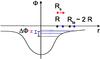 |
Fig. 1 The gravitational potential governing gas infall. As the DM outskirts develop (see Sect. 2), both the virial R and the turnaround radius Rta shift outwards, retaining the ratio Rta/R ≈ 2. Meanwhile, the outer potential becomes shallower and ΔΦ lower from the value marked in black to that in blue. The shock position Rs slowly outgrows R, lowering the drop to the value marked in red. |
On the ICP side, the outer gas will accrete with a lower infall speed
v1. As illustrated in Fig. 1, it is set to  by the outer gravitational
potential drop
by the outer gravitational
potential drop  . This is experienced
by successive shells of DM and gas that − after an initial expansion − turn around at
the radius Rta ≈ 2 R to begin their infall
toward the shock at Rs ≈ R. Thus the
potential drop
. This is experienced
by successive shells of DM and gas that − after an initial expansion − turn around at
the radius Rta ≈ 2 R to begin their infall
toward the shock at Rs ≈ R. Thus the
potential drop  (normalized
to the circular velocity
(normalized
to the circular velocity  at
r = R) reads as
at
r = R) reads as
 (2)This is seen (cf.
Fig. 1) to become shallower during
the outskirt’s development as ϵ exceeds 1, after which the approximation
Δφ ≈ (3 ϵ − 2)-1 ≈ (3ϵ)-1
applies.
(2)This is seen (cf.
Fig. 1) to become shallower during
the outskirt’s development as ϵ exceeds 1, after which the approximation
Δφ ≈ (3 ϵ − 2)-1 ≈ (3ϵ)-1
applies.
Actually, the shock position Rs slowly outgrows the virial R to approach Rta, and this yields an even lower effective potential drop (see Voit et al. 2003; Lapi et al. 2005). In fact, it can be shown that for ϵ > 1 the shock position may be approximated as Rs ≈ 2 R (1−4 ϵ-2), see Lapi et al. (2010); so from Eq. (2) we obtain Δφ ≈ 4 ϵ-2.
The direct and indirect effects of Ṁ dwindling combine into the
accretion rate scaling  , after which the infall
speed follows
, after which the infall
speed follows  (3)This is indeed
reduced strongly during the late development of the outskirts when both
Ṁ ∝ d/ϵ subsides and
Δφ ∝ ϵ-2 lowers, so that the overall
scaling
v1 ∝ d1/3/ϵ
applies for ϵ > 1; specifically, as ϵ increases
from 1 to 1.5 and then to 3, the prevailing Mach numbers decline from ℳ2 ≈ 10
to 6 and then to 3.
(3)This is indeed
reduced strongly during the late development of the outskirts when both
Ṁ ∝ d/ϵ subsides and
Δφ ∝ ϵ-2 lowers, so that the overall
scaling
v1 ∝ d1/3/ϵ
applies for ϵ > 1; specifically, as ϵ increases
from 1 to 1.5 and then to 3, the prevailing Mach numbers decline from ℳ2 ≈ 10
to 6 and then to 3.
These values are consistent with the Mach number distributions at low z sliced for flows of preheated gas into the cluster, as found by numerical simulations (e.g., Ryu et al. 2003; Skillman et al. 2008, see their Fig. 6 and Sect. 4; see also Vazza et al. 2010).
2.2. Weakening shocks and entropy demise
With v1 lowering toward transonic values, the shock strength
will eventually weaken. We recall (see Appendix B in Lapi et al. 2005) that the Rankine-Hugoniot
conservation conditions for a standing shock give the postshock temperatures and densities
in the form  (4)As the Mach number
decreases from values ℳ2 > 3 (defining strong shocks) to transonic
ℳ2 ≈ 1, the temperature ranges widely from
(4)As the Mach number
decreases from values ℳ2 > 3 (defining strong shocks) to transonic
ℳ2 ≈ 1, the temperature ranges widely from
 to
T2 ≃ T1, while the density
varies mildly from n2 ≃ 4 n1 to
n2 ≃ n1. Correspondingly, the
shock-generated entropy
to
T2 ≃ T1, while the density
varies mildly from n2 ≃ 4 n1 to
n2 ≃ n1. Correspondingly, the
shock-generated entropy  drops
from values
5 ℳ2 k1/42/3 16 ~
some 103 keV cm2 typical of strong shocks to intergalactic values
drops
from values
5 ℳ2 k1/42/3 16 ~
some 103 keV cm2 typical of strong shocks to intergalactic values
 keV cm2.
By the same token, the entropy outer ramp will abate. Its slope at the boundary has been
derived by Cavaliere et al. (2009) from the jumps
at the shock and the adjoining HE recalled in Sect. 1, to read as
 (5)Here,
![Mathematical equation: \hbox{$\mathcal{A} = 4\, (1+\epsilon/d)/[5+2\,(1+\epsilon/d)]\approx 1$}](/articles/aa/full_html/2011/01/aa15390-10/aa15390-10-eq108.png) applies as long as ϵ ≈ 1 and d ≈ 2/3 hold.
applies as long as ϵ ≈ 1 and d ≈ 2/3 hold.
However, the main dependence of aR on
ϵ and d is encased in
 through the boundary
temperature. We have just seen that
through the boundary
temperature. We have just seen that  holds as long as strong shock
conditions apply. If so,
bR ∝ 1/Δφ ∝ ϵ2
would rise fast as ϵ exceeds 1; but
holds as long as strong shock
conditions apply. If so,
bR ∝ 1/Δφ ∝ ϵ2
would rise fast as ϵ exceeds 1; but
 is meanwhile reduced
and the virial accretion shocks weakened, slowing down the net growth of
bR. The overall result is that
bR grows from the standard value 2.7 to
about 5 and then to about 8 while ϵ increases from 1 to 1.5 and then to
3.
is meanwhile reduced
and the virial accretion shocks weakened, slowing down the net growth of
bR. The overall result is that
bR grows from the standard value 2.7 to
about 5 and then to about 8 while ϵ increases from 1 to 1.5 and then to
3.
After Eq. (5), increasing values of bR cause aR to decrease, and imply progressive saturation and even a decline in the entropy produced at the boundary. Specifically, as ϵ increases from 1 to 1.5 and then to 3, the entropy slope aR goes from the standard value 1.1 to about 0 and then down to negative values around −2.
To tackle the issue, recall that, while the cluster outskirts develop to the currently observed radius R, the ICP is adiabatically compressed and settles into the DM potential well. Then the specific entropy k(r) stratifies shell by shell, leading to a running slope a(r) = aR that retains the sequence of the values set at the time of deposition (see Tozzi & Norman 2001; Lapi et al. 2005). As a result, on moving out from the early cluster body to the outskirts currently building up by secular accretion, the whole slope a(r) of the outer ramp decreases, and k(r) ∝ ra(r) flattens or even bends over.
To describe this behavior, in Lapi et al. (2010) we used an entropy slope a(r) = a − a′ (r − rb) smoothly decreasing from the body value a ≈ 1.1. We found a value a ≈ 0 at r ≈ R/2 and values a ≈ −2 at R (as illustrated in Fig. 1 of Lapi et al. 2010), consistently with the data by Bautz et al. (2009) and George et al. (2009).
2.3. Onset of turbulence
Here we show that such an entropy demise due to Ṁ dwindling will arise
together with the onset of turbulence triggered by shock weakening. In
fact, the latter causes the postshock speeds,
 (6)to grow from
values around 1/4 and approach 1. With
v1 ∝ ϵ-1 lowering sharply while
c1 varies as (1 + z) or less, the kinetic
energy ratio is thus enhanced relative to the strong shock value 6.3%,
see Sect. 2.1. For example, as ϵ grows from 1 to 1.5 and then to 3−5,
the ratio
(6)to grow from
values around 1/4 and approach 1. With
v1 ∝ ϵ-1 lowering sharply while
c1 varies as (1 + z) or less, the kinetic
energy ratio is thus enhanced relative to the strong shock value 6.3%,
see Sect. 2.1. For example, as ϵ grows from 1 to 1.5 and then to 3−5,
the ratio  increases
from 10% to 14% and then to 25−39%. The ratio
increases
from 10% to 14% and then to 25−39%. The ratio  of the
residual bulk to the sound’s speed past the shock also increases for decreasing
ℳ2; in particular, it goes from 25% to 50% as ℳ2 ranges from 1
to 3−5. On average, for a CC cluster we find the condition
ℳ2 ∝ d1/3/ ⟨ ϵ(z) ⟩ (1 + z) ≲ 3
for shock weakening to be met at redshifts z ≲ 0.3, on using for the
average ⟨ ϵ ⟩ the values given by Lapi
& Cavaliere (2009) in their Fig. 6. In a nutshell, combining Eqs. (4)
and (6) yields an inverse relation of
with k2/k1.
of the
residual bulk to the sound’s speed past the shock also increases for decreasing
ℳ2; in particular, it goes from 25% to 50% as ℳ2 ranges from 1
to 3−5. On average, for a CC cluster we find the condition
ℳ2 ∝ d1/3/ ⟨ ϵ(z) ⟩ (1 + z) ≲ 3
for shock weakening to be met at redshifts z ≲ 0.3, on using for the
average ⟨ ϵ ⟩ the values given by Lapi
& Cavaliere (2009) in their Fig. 6. In a nutshell, combining Eqs. (4)
and (6) yields an inverse relation of
with k2/k1.
These postshock flows provide bounds to the energy level of subsonic turbulent motions that is driven by smooth accretion in relaxed clusters. Minor, intermittent, and localized contributions may be added by the complementary clumpy component of the accretion, recently re-calibrated to less than 30% in the outskirts of relaxed halos (see Fakhouri et al. 2010; Genel et al. 2010; Wang et al. 2010). Our bounds actually constitute fair estimates of the amplitudes of outer turbulent energy at r ~ R, as shown by similar values obtained both observationally (see Mahdavi et al. 2008; Zhang et al. 2010) and in many numerical simulations from Evrard (1990) to Lau et al. (2009).
3. Modeling the turbulent support
Turbulent motions start at the virial radius R with comparable coherence
lengths L ~ R/2, set in relaxed CC clusters by
the pressure scale height or by shock segmentation (see Iapichino & Niemeyer 2008; Ryu et al.
2008; Pfrommer & Jones 2010; Valdarnini 2010; Vazza
et al. 2010). Then they fragment downstream into a dispersive cascade over the
“inertial range”, to sizes ℓ where dissipation begins after the classic
picture by Kolmogorov (1941), Obukhov (1941), and Monin &
Yaglom (1965). In the ICP context the dissipation scale (equivalently to the
classic Reynolds’ scaling) writes as  in
terms of the ion collisional mean free path λpp and of the ratio
in
terms of the ion collisional mean free path λpp and of the ratio
 of the turbulent rms
speed to the sound’s, see Inogamov & Sunyaev
(2003). For subsonic turbulence with
of the turbulent rms
speed to the sound’s, see Inogamov & Sunyaev
(2003). For subsonic turbulence with  (see
direct observational bounds by Schücker et al. 2004;
Sanders et al. 2010, and references therein) the
relevant scale ℓ somewhat exceeds
λpp ~ 102 kpc.
(see
direct observational bounds by Schücker et al. 2004;
Sanders et al. 2010, and references therein) the
relevant scale ℓ somewhat exceeds
λpp ~ 102 kpc.
In the presence of outer magnetic fields B ≲ 10-1 μG (see Bonafede et al. 2010; Pfrommer & Jones 2010; also Ryu et al. 2008), the key − if quantitatively debated − feature is their degree of tangling; then the effective mean free path is provided by the coherence scale of the field, which is somewhat larger than λpp (see discussions by Narayan & Medvedev 2001; Inogamov & Sunyaev 2003; Govoni et al. 2006; Brunetti & Lazarian 2007).
Clearly the above estimates provide useful guidelines, but need theoretical modeling and observational probing. Both issues are addressed next. Since turbulent motions contribute to the pressure (see Landau & Lifshitz 1959) to sustain HE, our modeling focuses on the ratio δ(r) ≡ pnth/pth of turbulent to thermal pressure (or, equivalently, on the ratio δ/(1 + δ) of turbulent to total pressure), with radial shape decaying on the scale ℓ from the boundary value δR.
The total pressure is conveniently and generally written as
pth(r) [1 + δ(r)] ,
while the thermal component is still expressed as
pth(r) ∝ k(r) n5/3(r).
With this addition, we proceed by solving the HE equation just along the steps leading to
Eq. (1), and now find the temperature profile in the form
![Mathematical equation: \begin{eqnarray} \nonumber{T(r)\over T_R}&=&\left[{k(r)\over k_R}\right]^{3/5}\, \left[{1+\delta_R\over 1+\delta(r)}\right]^{2/5}\,\left\{1+{2\over 5}\, {b_R\over 1+\delta_R}\, \right.\\ &&\times \left.\int^R_r{\mathrm{d} x\over x}\,{v_{\rm c}^2(x)\over v_R^2}\, \left[{k_R\over k(x)}\right]^{3/5}\, \left[{1+\delta_R\over 1+\delta(x)}\right]^{3/5}\right\}, \end{eqnarray}](/articles/aa/full_html/2011/01/aa15390-10/aa15390-10-eq165.png) (7)which
extends Eq. (1) for δ > 0. Again,
n(r) is linked to T(r)
by
n = [kBT/k] 3/2.
(7)which
extends Eq. (1) for δ > 0. Again,
n(r) is linked to T(r)
by
n = [kBT/k] 3/2.
The actual temperature at the boundary is now lowered to TR = T2/(1 + δR). This is seen from Rankine-Hugoniot conditions in the presence of turbulent pressure; the latter obviously implies the term p2 (1 + δR) to be added on the righthand side of the stress balance, and the corresponding one 5 p2 (1 + δR) v2/2 in the energy flow (see Eqs. (B1) in Lapi et al. 2005).
In our numerical computations that follow we adopt for fully developed turbulence the
simple functional shape (rather than a constant δ as used by Bode et al. 2009)
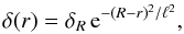 (8)which decays on the
scale ℓ inward of a round maximum, a smoothed-out
representation of the inertial range. This is illustrated in Fig. 2 for three cases with ℓ = 0.9 R,
ℓ = 0.5 R, and
ℓ = 0.2 R. The runs
δ(r) we adopt are consistent with those recently
indicated by numerical simulations (e.g., Lau et al.
2009).
(8)which decays on the
scale ℓ inward of a round maximum, a smoothed-out
representation of the inertial range. This is illustrated in Fig. 2 for three cases with ℓ = 0.9 R,
ℓ = 0.5 R, and
ℓ = 0.2 R. The runs
δ(r) we adopt are consistent with those recently
indicated by numerical simulations (e.g., Lau et al.
2009).
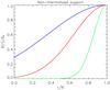 |
Fig. 2 Nonthermalized pressure support δ(r) ≡ pnth/pth normalized to the boundary value δR computed after Eq. (8). The blue line refers to ℓ = 0.9 R, red line to ℓ = 0.5 R, and green line to ℓ = 0.2 R. |
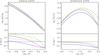 |
Fig. 3 Profiles of pressure and temperature computed with the SM. The dashed line illustrates the pure thermal (laminar) case, while solid lines illustrate the turbulent case with δR = 40% and different ℓ (color code as in Fig. 2). In the left panel, solid lines refer to the thermal pressure, dotted ones to the total pressure. |
4. Results
We illustrate the resulting temperature and pressure profiles in Fig. 3. Relative to pure thermal HE with δR = 0, in the outskirts the thermal pressure lowers since it is helped by turbulent motions in sustaining the equilibrium, while the pressure run is moderately steeper. At the center, the pressure is mainly contributed by the thermal component.
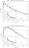 |
Fig. 4 Profiles of projected X-ray temperature (brightness in the insets) for the CC clusters A1689 (top) and A1795 (bottom). Data are from Snowden et al. (2008) with XMM-Newton (circles), and from Bautz et al. (2009) and Kawaharada et al. (2010) with Suzaku (squares). The solid lines represent our best fits with the SM extended to include turbulence after Eqs. (7) and (8) with δR = 40% and ℓ = 0.5 R. The dashed ones illustrate the outcomes in the absence of turbulence, but still with entropy decreasing outwards as in Lapi et al. (2010). For comparison, the dotted lines illustrate the case with an uniform entropy slope. |
It is seen that the variations in temperature (with the classic CC shape) are mild, and primarily stem from the reduction of TR/T2 by the factor 1 + δR = 1.4 discussed in Sect. 3. Thus we recognize the saturation or bending over of entropy on scales r ≲ R/2 (see Sect. 2) to constitute the primary cause of the steep temperature profiles observed by Suzaku. These drop by factors around 10 from the peak to the outer boundary in the low-z clusters like A1795 and PKS0745-191.
This view is confirmed by Fig. 4, where we illustrate our best fits with the SM to the temperature and surface brightness profiles for the two clusters A1795 (north sector) and A1689 (azimutally averaged), one at a low and the other at a relatively high z. The figure shows that the SM with an entropy slope decreasing through the outskirts from standard values a ≈ 1.1 at r < R/2 to a ≈ −1.8 at R (just as expected in Sect. 2.2) fits the temperature profile of the low-z cluster A1795 much better than the case with uniform slope a ≈ 1.1. As expected, the difference is barely discernible for the relatively high-z cluster A1689. Both fits are only mildly affected when including in the SM the turbulent support. The linked n(r) profiles flatten out to enhanced brightness landings (cf. insets in Fig. 4), a simple warning of interesting temperature and turbulence distributions.
A far-reaching consequence of turbulent support shows up (see Fig. 5, left) in the reconstructions of DM masses from X-ray observables based on reversing the thermal HE equation (cf. Sarazin 1988, p. 92). It is seen that the mass reconstructed when ignoring the nonthermalized component deviates from the true mass by different amounts, and for low values of the dissipation scale ℓ may even have a non-monotonic behavior, not unlike the results by Kawaharada et al. (2010) in three sectors of A1689 (cf. their Fig. 8). In all cases, the reconstructed mass within R is negatively biased by 20−30% relative to the true one. Accounting for such a bias constitutes a key point to resolve the tension between weak lensing and X-ray masses (e.g., Nagai et al. 2007; Lau et al. 2009; Meneghetti et al. 2010), and in deriving precise cosmological parameters from statistics of cluster masses via the fast X-ray observations (see Vikhlinin et al. 2009).
The above picture may be double-checked in individual clusters by directly gauging with the SZ scattering how the electron pressures are lowered in the presence of outer turbulence. In Fig. 5 (right) it is seen that along the line of sight running mainly into the outskirts, we expect the latter to be 20−30% lower than the pure thermal case. This is stronger by a factor of about 5 than the effects from delayed equipartition between electron and ion temperatures downstream of the shock over the relevant mean free path. A corresponding reduction is implied in the requirements for sensitivity and/or observation times with upcoming sophisticated instruments like ALMA (see Wong & Sarazin 2009). Meanwhile, statistical evidence of SZ reductions has been extracted from stacked data by Komatsu et al. (2010).
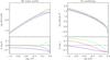 |
Fig. 5 Left: profile of DM mass. The dashed line illustrates the true mass, while the solid lines illustrate what is reconstructed from X-ray observables on assuming pure thermal HE. Right: projected profile of SZ scattering; the dashed line refers to the purely thermal case, while solid lines refer to the turbulent case. In both panels δR = 40% and different values of ℓ (color code as in Fig. 2) are adopted. |
5. Discussion and conclusions
To answer the issue raised at the end of Sect. 1, we investigated the connection of ICP
turbulence in cluster outskirts with virial accretion shocks. Among the variety of shocks
found in numerical simulations, these are most amenable to a simple treatment, which may
also shed light on more complex conditions. A result to stress is the inverse
nature of the connection that follows from combining the key Eqs. (4) and (6): as
the Mach number ℳ of the shock decreases, the postshock entropy
 lowers with ℳ2, while the residual bulk energy
rises with
ℳ-2. In other words, saturation of entropy production and
increasing bulk flows to drive turbulence occur
together.
lowers with ℳ2, while the residual bulk energy
rises with
ℳ-2. In other words, saturation of entropy production and
increasing bulk flows to drive turbulence occur
together.
To pinpoint when this is bound to occur, we base on the quantity
 including three
factors: the infall speed
including three
factors: the infall speed  , see Eq. (3); the
accretion rate Ṁ ∝ d/ϵ; and the
residual kinetic energy ratio , see Eq. (6) and
discussion thereafter. Such a quantity depends strongly on
d and even more on ϵ, which render the effects on the
outskirt’s growth of the cosmological expansion accelerated by the dark energy, and of the
declining shape of the initial DM perturbation wings, respectively.
, see Eq. (3); the
accretion rate Ṁ ∝ d/ϵ; and the
residual kinetic energy ratio , see Eq. (6) and
discussion thereafter. Such a quantity depends strongly on
d and even more on ϵ, which render the effects on the
outskirt’s growth of the cosmological expansion accelerated by the dark energy, and of the
declining shape of the initial DM perturbation wings, respectively.
This leads us to predict that the turbulent support starts to increase on average for
z < 1/2 during the late development of the cluster outskirts
when d ≈ 1/2 and ϵ > 1 apply. Then turbulence
briskly rises at z ≲ 0.3 when the shocks become transonic.
On the other hand, environmental (even anisotropic) variance is introduced when the residual
energy flow  , strongly
dependent on ϵ, is modulated by the adjacent filament/void structure. At
very low z, a high level of thermal support will persist in sectors
adjacent to filaments, as is apparently the case with A1795 and PKS0745-191 (see Bautz et al. 2009; George
et al. 2009). By the same token, values ϵ > 1 will prevail
in cluster sectors facing a void, causing an early onset of turbulence there given
sufficient Ṁ. Meanwhile, in neighboring sectors facing a filament, values
ϵ ≈ 1 still hold and the thermal support may still prevail, a condition
that apparently applies to A1689 (see Kawaharada et al.
2010; Molnar et al. 2010).
, strongly
dependent on ϵ, is modulated by the adjacent filament/void structure. At
very low z, a high level of thermal support will persist in sectors
adjacent to filaments, as is apparently the case with A1795 and PKS0745-191 (see Bautz et al. 2009; George
et al. 2009). By the same token, values ϵ > 1 will prevail
in cluster sectors facing a void, causing an early onset of turbulence there given
sufficient Ṁ. Meanwhile, in neighboring sectors facing a filament, values
ϵ ≈ 1 still hold and the thermal support may still prevail, a condition
that apparently applies to A1689 (see Kawaharada et al.
2010; Molnar et al. 2010).
With the closer focus provided by the SM, we find that while the shocks weaken not only the boundary entropy production saturates but also the whole outer entropy distribution k(r) flattens and the temperature profiles T(r) become steeper, and do so consistently with the observations. Eventually, as the inflow approaches the transonic regime, k(r) tends to bend over and T(r) to steepen somewhat more.
But then subsonic turbulence arises at the boundary. Its inner distribution follows the classic picture of the turbulent motion fragmentation, with a scale for its final dissipation which is still debated. This demands closer probing, which we have tackled with the fast, analytic tool provided by the SM. The present data from joint X-ray and weak lensing observations (see Kawaharada et al. 2010; Molnar et al. 2010; Zhang et al. 2010) concur with simulations (see Lau et al. 2009) to show no evidence of a dissipation scale that is much shorter than ~102 kpc, conceivably set by tangling of the magnetic field (see discussions by Narayan & Medvedev 2001; Brunetti & Lazarian 2007).
To summarize, in the outskirts of relaxed clusters we find the following.
-
Turbulence is related to weakening shocks at late cosmic epochsz < 0.3, when saturation of entropy production causes steep temperature profiles.
-
Turbulent excess pressures δR = pnth/pth up to 40% arise at the boundary, declining inwards on scales of ℓ ~ 100 kpc.
-
The overall masses derived from X-rays are necessarily biased low, down to 20−30% when such a turbulent support is ignored. These findings are consistent with the current observational and numerical data. Moreover, we predict that
-
variance concerning steep T(r) and turbulent support in cluster sectors will be correlated with the filament modulation of the adjacent environment,
-
the SZ scattering will be considerably lowered relative to the pure thermal case, along the lines of sight running mainly into the outskirts or their sectors where X-rays concur with lensing data in signaling turbulent support.
A final comment concerns the giant radiohalos observed in the centers of several clusters to emit synchrotron radiation. These suggest that nonthermal support may be contributed by a mixture of magnetic field and relativistic particles accelerated by shocks and turbulence due to mergers (see Brunetti et al. 2007; Biermann et al. 2009; Brunetti et al. 2009). With their limited acceleration efficiency and short persistence, these processes are apparently widespread in NCC clusters, mainly at z > 0.2, so they have minimal superposition or interference with the substantial, low-z, long-lived, outer turbulent component concerning mainly CCs, which we have addressed here.
The picture we pursue envisages the infall kinetic energy to thermalize along two channels. First, supersonic inflows achieve thermalization at the shock transition via a sharp jump (or a few jumps within a layer of limited thickness, see Lapi et al. 2005). Second, the subsonic turbulent motions left over downstream of the shocks, particularly downstream of weak shocks, are dispersed into a cascade of many effective degrees of freedom (see Landau & Lifshitz 1959), down to scales where dissipation becomes effective. The channels’ branching ratio shifts toward the latter when the shock weakens, for z ≲ 0.3; meanwhile, turbulence concurs with thermal pressure to support the ICP equilibrium in the outskirts. The picture substantiates the following formal remark: Eq. (7) corresponds to Eq. (1) for the variable T (1 + δ) in terms of the extended entropy k (1 + δ).
This picture of onset and development of outer ICP turbulence may be fruitful in other contexts, in particular for shocks and turbulence in wakes around mergers. Thus it warrants close modeling with our fast yet precise analytic SM, to probe the key turbulence features, amplitude and scale, over wide cluster samples in a range of z.
R/2 ≈ R500 ≈ 2 R200/3 holds in terms of the radii inside which the average DM overdensity relative to the critical universe amounts to 500 and 200, respectively.
Acknowledgments
This work was supported by ASI and INAF. We thank our referee for helpful comments and suggestions. A.L. thanks SISSA and INAF-OATS for their warm hospitality.
References
- Bautz, M. W., Miller, E. D., Sanders, J. S., et al. 2009, PASJ, 61, 1117 [NASA ADS] [Google Scholar]
- Biermann, P. L., Becker, J. K., Caramete, L., et al. 2009, Nucl. Phys. Supp., 190, 61B [Google Scholar]
- Binney, J. 1974, MNRAS, 168, 73 [NASA ADS] [Google Scholar]
- Birkinshaw, M., & Lancaster, K. 2007, NewAR, 51, 346 [Google Scholar]
- Bode, P., Ostriker, J. P., & Vikhlinin, A. 2009, ApJ, 700, 989 [NASA ADS] [CrossRef] [Google Scholar]
- Bonafede, A., Feretti, L., Murgia, M., et al. 2010, A&A, 513, A30 [NASA ADS] [CrossRef] [EDP Sciences] [Google Scholar]
- Brunetti, G., & Lazarian, A. 2007, MNRAS, 378, 245 [NASA ADS] [CrossRef] [Google Scholar]
- Brunetti, G., Venturi, T., Dallacasa, D., et al. 2007, ApJ, 670, L5 [NASA ADS] [CrossRef] [Google Scholar]
- Brunetti, G., Cassano, R., Dolag, K., & Setti, G. 2009, A&A, 507, 661 [NASA ADS] [CrossRef] [EDP Sciences] [Google Scholar]
- Cavagnolo, K., Donahue, M., Voit, G. M., & Sun, M. 2009, ApJS, 182, 12 [NASA ADS] [CrossRef] [Google Scholar]
- Cavaliere, A., Lapi, A., & Menci, N. 2002, ApJ, 581, L1 [NASA ADS] [CrossRef] [Google Scholar]
- Cavaliere, A., Lapi, A., & Fusco-Femiano, R. 2009, ApJ, 698, 580 [NASA ADS] [CrossRef] [Google Scholar]
- Doroshkevich, A. G. 1973, SvA, 16, 986 [NASA ADS] [Google Scholar]
- Evrard, A. E. 1990, ApJ, 363, 349 [NASA ADS] [CrossRef] [Google Scholar]
- Fakhouri, O., Ma, C.-P., & Boylan-Kolchin, M. 2010, MNRAS, 406, 2267 [NASA ADS] [CrossRef] [Google Scholar]
- Fusco-Femiano, R., Cavaliere, A., & Lapi, A. 2009, ApJ, 705, 1019 [NASA ADS] [CrossRef] [Google Scholar]
- Genel, S., Bouché, N., Naab, T., Sternberg, A., & Genzel, R. 2010, ApJ, 719, 229 [NASA ADS] [CrossRef] [Google Scholar]
- George, M. R., Fabian, A. C., Sanders, J. S., Young, A. J., & Russell, H. R. 2009, MNRAS, 395, 657 [NASA ADS] [CrossRef] [Google Scholar]
- Giacconi, R., et al. 2009, in Astro2010: The Astronomy and Astrophysics Decadal Survey (Science White Papers), 90 [Google Scholar]
- Govoni, F., Murgia, M., Feretti, L., et al. 2006, A&A, 460, 425 [NASA ADS] [CrossRef] [EDP Sciences] [Google Scholar]
- Hoshino, A., Patrick Henry, J., Sato, K., et al. 2010, PASJ, 62, 371 [NASA ADS] [CrossRef] [Google Scholar]
- Iapichino, L., & Niemeyer, J. C. 2008, MNRAS, 388, 1089 [NASA ADS] [CrossRef] [Google Scholar]
- Inogamov, N. A., & Sunyaev, R. A. 2003, AstL, 29, 791 [Google Scholar]
- Kawaharada, M., Okabe, N., Umetsu, K., et al. 2010, ApJ, 714, 423 [NASA ADS] [CrossRef] [Google Scholar]
- Kolmogorov, A. 1941, Dokl. Akad. Nauk SSSR, 30, 301 [Google Scholar]
- Komatsu, E., Smith, K. M., Dunkley, J., et al. 2010, ApJS, accepted [arXiv:1001.4538] [Google Scholar]
- Landau, L. D., & Lifshitz, E. M. 1959, Fluid Mechanics (Oxford: Pergamon) [Google Scholar]
- Lapi, A., & Cavaliere, A. 2009, ApJ, 692, 174 [NASA ADS] [CrossRef] [Google Scholar]
- Lapi, A., Cavaliere, A., & Menci, N. 2005, ApJ, 619, 60 [NASA ADS] [CrossRef] [Google Scholar]
- Lapi, A., Fusco-Femiano, R., & Cavaliere, A. 2010, A&A, 516, A34 [NASA ADS] [CrossRef] [EDP Sciences] [Google Scholar]
- Lau, E. T., Kravtsov, A. V., & Nagai, D. 2009, ApJ, 705, 1129 [NASA ADS] [CrossRef] [Google Scholar]
- Lu, Y., Mo, H. J., Katz, N., & Weinberg, M. D. 2006, MNRAS, 368, 1931 [NASA ADS] [CrossRef] [Google Scholar]
- Mahdavi, A., Hoekstra, H., Babul, A., & Henry, J. P. 2008, MNRAS, 384, 1567 [NASA ADS] [CrossRef] [Google Scholar]
- Markevitch, M., & Vikhlinin, A. 2007, Phys. Rep., 443, 1 [NASA ADS] [CrossRef] [EDP Sciences] [Google Scholar]
- McCarthy, I. G., Bower, R. G., Balogh, M. L., et al. 2007, MNRAS, 376, 497 [NASA ADS] [CrossRef] [Google Scholar]
- McNamara, B. R., & Nulsen, P. E. J. 2007, ARA&A, 45, 117 [NASA ADS] [CrossRef] [MathSciNet] [Google Scholar]
- Meneghetti, M., Rasia, E., Merten, J., et al. 2010, A&A, 514, A93 [NASA ADS] [CrossRef] [EDP Sciences] [Google Scholar]
- Molendi, S., & Pizzolato, F. 2001, ApJ, 560, 194 [NASA ADS] [CrossRef] [Google Scholar]
- Molnar, S. M., Chiu, I.-N., Umetsu, K., et al. 2010, ApJ, 724, L1 [NASA ADS] [CrossRef] [Google Scholar]
- Monin, A. S., & Yaglom, A. M. 1965, Statistical Hydromechanics (Nauka: Moscow) [Google Scholar]
- Narayan, R., & Medvedev, M. V. 2001, ApJ, 562, L129 [NASA ADS] [CrossRef] [Google Scholar]
- Obukhov, A. M. 1941, Dokl. Akad. Nauk. SSSR, 1, 22 [Google Scholar]
- Nagai, D., Kravtsov, A. V., & Vikhlinin, A. 2007, ApJ, 668, 1 [NASA ADS] [CrossRef] [Google Scholar]
- Paul, S., Iapichino, L., Miniati, F., Bagchi, J., & Mannheim, K. 2010, ApJ, submitted [arXiv:1001.1170] [Google Scholar]
- Pfrommer, C., & Jones, T. W. 2010, ApJ, submitted [arXiv:1004.3540] [Google Scholar]
- Pratt, G. W., Arnaud, M., Piffaretti, R., et al. 2010, A&A, 511, A85 [NASA ADS] [CrossRef] [EDP Sciences] [Google Scholar]
- Reiprich, T. H., Hudson, D. S., Zhang, Y.-Y., et al. 2009, A&A, 501, 899 [NASA ADS] [CrossRef] [EDP Sciences] [Google Scholar]
- Ricker, P. M., & Sarazin, C. L. 2001, ApJ, 561, 621 [NASA ADS] [CrossRef] [Google Scholar]
- Ryu, D., Kang, H., Hallman, E., & Jones, T. W. 2003, ApJ, 593, 599 [NASA ADS] [CrossRef] [Google Scholar]
- Ryu, D., Kang, H., Cho, J., Das, S., et al. 2008, Science, 320, 909 [NASA ADS] [CrossRef] [PubMed] [Google Scholar]
- Sanders, J. F., Fabian, A. C., & Smith, R. K. 2010, MNRAS, in press [arXiv:1008.3500] [Google Scholar]
- Sarazin, C. L. 1988, X-ray Emission from Clusters of Galaxies (Cambridge: Cambridge Univ. Press) [Google Scholar]
- Schäfer, M., & Bartelmann, M. 2007, MNRAS, 377, 253 [NASA ADS] [CrossRef] [Google Scholar]
- Schücker, P., Finoguenov, A., Miniati, F., Böhringer, H., & Briel, U. G. 2004, A&A, 426, 387 [NASA ADS] [CrossRef] [EDP Sciences] [Google Scholar]
- Skillman, S. W., O’Shea, B. W., Hallman, E. J., Burns, J. O., & Norman, M. L. 2008, ApJ, 689, 1063 [NASA ADS] [CrossRef] [Google Scholar]
- Snowden, S. L., Mushotzky, R. F., Kuntz, K. D., & Davis, D. S. 2008, A&A, 478, 615 [NASA ADS] [CrossRef] [EDP Sciences] [Google Scholar]
- Sunyaev, R. A., & Zeldovich, Ya. B. 1972, A&A, 20, 189 [NASA ADS] [Google Scholar]
- Tozzi, P., & Norman, C. 2001, ApJ, 546, 63 [NASA ADS] [CrossRef] [Google Scholar]
- Valageas, P., & Silk, J. 1999, A&A, 350, 725 [NASA ADS] [Google Scholar]
- Valdarnini, R. 2010, A&A, in press [arXiv:1010.3378] [Google Scholar]
- Vazza, F., Brunetti, G., Gheller, C., & Brunino, R. 2010, New Astron., 15, 695 [NASA ADS] [CrossRef] [Google Scholar]
- Vikhlinin, A., Kravtsov, A. V., Burenin, R. A., et al. 2009, ApJ, 692, 1060 [NASA ADS] [CrossRef] [Google Scholar]
- Voit, G. M. 2005, Rev. Mod. Phys., 77, 207 [NASA ADS] [CrossRef] [Google Scholar]
- Voit, G. M., Balogh, M. L., Bower, R. G., et al. 2003, ApJ, 593, 272 [NASA ADS] [CrossRef] [Google Scholar]
- Wang, J., Navarro, J. F., Frenk, C. S., et al. 2010, MNRAS, submitted [arXiv:1008.5114] [Google Scholar]
- Weinberg, S. 2008, Cosmology (Oxford: Oxford Univ. Press) [Google Scholar]
- Wong, K.-W., & Sarazin, C. L. 2009, ApJ, 707, 1141 [NASA ADS] [CrossRef] [Google Scholar]
- Wu, K. K. S., Fabian, A. C., & Nulsen, P. E. J. 2000, MNRAS, 318, 889 [NASA ADS] [CrossRef] [Google Scholar]
- Zhang, Y.-Y., Okabe, N., Finoguenov, A., et al. 2010, ApJ, 711, 1033 [NASA ADS] [CrossRef] [Google Scholar]
- ZuHone, J. A., Markevitch, M., & Johnson, R. E. 2010, ApJ, 717, 908 [NASA ADS] [CrossRef] [Google Scholar]
All Figures
|
Fig. 1 The gravitational potential governing gas infall. As the DM outskirts develop (see Sect. 2), both the virial R and the turnaround radius Rta shift outwards, retaining the ratio Rta/R ≈ 2. Meanwhile, the outer potential becomes shallower and ΔΦ lower from the value marked in black to that in blue. The shock position Rs slowly outgrows R, lowering the drop to the value marked in red. |
| In the text | |
|
Fig. 2 Nonthermalized pressure support δ(r) ≡ pnth/pth normalized to the boundary value δR computed after Eq. (8). The blue line refers to ℓ = 0.9 R, red line to ℓ = 0.5 R, and green line to ℓ = 0.2 R. |
| In the text | |
|
Fig. 3 Profiles of pressure and temperature computed with the SM. The dashed line illustrates the pure thermal (laminar) case, while solid lines illustrate the turbulent case with δR = 40% and different ℓ (color code as in Fig. 2). In the left panel, solid lines refer to the thermal pressure, dotted ones to the total pressure. |
| In the text | |
|
Fig. 4 Profiles of projected X-ray temperature (brightness in the insets) for the CC clusters A1689 (top) and A1795 (bottom). Data are from Snowden et al. (2008) with XMM-Newton (circles), and from Bautz et al. (2009) and Kawaharada et al. (2010) with Suzaku (squares). The solid lines represent our best fits with the SM extended to include turbulence after Eqs. (7) and (8) with δR = 40% and ℓ = 0.5 R. The dashed ones illustrate the outcomes in the absence of turbulence, but still with entropy decreasing outwards as in Lapi et al. (2010). For comparison, the dotted lines illustrate the case with an uniform entropy slope. |
| In the text | |
|
Fig. 5 Left: profile of DM mass. The dashed line illustrates the true mass, while the solid lines illustrate what is reconstructed from X-ray observables on assuming pure thermal HE. Right: projected profile of SZ scattering; the dashed line refers to the purely thermal case, while solid lines refer to the turbulent case. In both panels δR = 40% and different values of ℓ (color code as in Fig. 2) are adopted. |
| In the text | |
Current usage metrics show cumulative count of Article Views (full-text article views including HTML views, PDF and ePub downloads, according to the available data) and Abstracts Views on Vision4Press platform.
Data correspond to usage on the plateform after 2015. The current usage metrics is available 48-96 hours after online publication and is updated daily on week days.
Initial download of the metrics may take a while.