| Issue |
A&A
Volume 691, November 2024
|
|
|---|---|---|
| Article Number | A73 | |
| Number of page(s) | 11 | |
| Section | Astrophysical processes | |
| DOI | https://doi.org/10.1051/0004-6361/202451903 | |
| Published online | 30 October 2024 | |
Electromagnetic signatures of black hole clusters in the center of super-Eddington galaxies
1
Instituto Argentino de Radioastronomía (CCT La Plata, CONICET; CICPBA; UNLP), C.C.5, (1894), Villa Elisa, Argentina
2
Facultad de Ciencias Astronómicas y Geofísicas, Universidad Nacional de La Plata, B1900FWA La Plata, Argentina
⋆ Corresponding author; leandroabaroa@gmail.com
Received:
16
August 2024
Accepted:
3
September 2024
Supermassive black holes (SMBHs) at the centers of active galaxies are fed by accretion disks that radiate from the infrared or optical to the X-ray bands. Several types of objects can orbit SMBHs, including massive stars, neutron stars, clouds from the broad- and narrow-line regions, and X-ray binaries. Isolated black holes with a stellar origin (BHs of ∼10 M⊙) should also be present in large numbers within the central parsec of the galaxies. These BHs are expected to form a cluster around the SMBH as a result of the enhanced star formation rate in the inner galactic region and the BH migration caused by gravitational dynamical friction. However, except for occasional microlensing effects on background stars or gravitational waves from binary BH mergers, the presence of a BH population is hard to verify. In this paper, we explore the possibility of detecting electromagnetic signatures of a central cluster of BHs when the accretion rate onto the central SMBH is greater than the Eddington rate. In these supercritical systems, the accretion disk launches powerful winds that interact with the objects orbiting the SMBH. Isolated BHs can capture matter from this dense wind, leading to the formation of small accretion disks around them. If jets are produced in these single microquasars, they could be sites of particle acceleration to relativistic energies. These particles in turn are expected to cool by various radiative processes. Therefore, the wind of the SMBH might illuminate the BHs through the production of both thermal and nonthermal radiation.
Key words: accretion, accretion disks / radiation mechanisms: general / stars: black holes / stars: jets / galaxies: active / galaxies: nuclei
© The Authors 2024
 Open Access article, published by EDP Sciences, under the terms of the Creative Commons Attribution License (https://creativecommons.org/licenses/by/4.0), which permits unrestricted use, distribution, and reproduction in any medium, provided the original work is properly cited.
This article is published in open access under the Subscribe to Open model. Subscribe to A&A to support open access publication.
1. Introduction
Supermassive black holes (SMBHs) at the centers of active galaxies are fed by accretion disks that radiate from the optical band to the X-rays. In many cases, a dusty torus obscures the central region and emits mainly in the infrared.
Various types of objects can orbit the SMBHs at the centers of galaxies, including massive stars (Bahcall & Wolf 1976), neutron stars (Kim & Davies 2018), clouds from broad- and narrow-line regions (Müller & Romero 2020; Sotomayor & Romero 2022), and X-ray binaries (Hailey et al. 2018; Mori et al. 2021). Isolated black holes with a stellar origin (BHs of ∼10 M⊙) should also be present in large numbers within the central parsec of most galaxies. These BHs are expected to form a cluster around the SMBH as a result of the enhanced star formation rate in the inner galaxy and BH migration caused by gravitational dynamical friction (Miralda-Escudé & Gould 2000; McKernan et al. 2011; Girma & Loeb 2019). However, except for occasional microlensing effects on background stars (Chanamé et al. 2001) or gravitational waves from BH binary mergers (Rasskazov & Kocsis 2019; Gondán & Kocsis 2022; Gaete et al. 2024), the presence of a BH population is hard to verify. Observational signatures associated with the accretion of matter onto the BHs may provide clues for identifying them.
Accretion of matter onto BHs on all scales proceeds in three basic regimes, depending on the relation of the actual accretion rate  to the Eddington rate
  : a highly sub-Eddington regime,
  (Narayan & Yi 1994); a moderate sub-Eddington regime,
  (Shakura & Sunyaev 1973); and a super-Eddington regime,
  (Abramowicz et al. 1980; Fukue 2004). In the last regime, the radiation pressure overcomes gravity in the innermost part of the disk, which becomes geometrically and optically thick. The surface layers of the disk are ejected as a consequence of the self-regulation of the BH accretion at the Eddington rate (Fukue 2009; Tomida et al. 2015; Abaroa et al. 2023). Two examples of super-Eddington accretion systems involving stellar BHs are ultraluminous X-ray sources (e.g. NGC4190 X-1, see Abaroa et al. 2023; Combi et al. 2024) and some microquasars, such as the Galactic SS433 (Fabrika 2004). SMBHs can also accrete at supercritical rates in some cases (e.g. Mrk 335, Sotomayor & Romero 2022).
The actual fraction of supercritical SMBHs in the galaxies is not well known (see Du et al. 2016, 2018; Liu et al. 2021, for some samples). In these systems, the accretion disk surrounding the central SMBH launches powerful winds with mass-loss rates similar to the accretion rate. In particular, when the SMBH has a relatively low mass, ≲107 M⊙, it can disrupt stars by tidal forces (in a tidal disruption event; TDE) triggering supercritical (De Colle et al. 2012; Stone & Metzger 2016; Tadhunter et al. 2017; Zubovas 2019; Dai et al. 2021; Kaur & Stone 2024; Price et al. 2024) or hypercritical accretion regimes with  in the most extreme cases (Inayoshi et al. 2016; Sakurai et al. 2016; Takeo et al. 2020). These strong outflows then interact with the objects orbiting the SMBH on their way out of the system.
Isolated BHs from the central cluster can capture matter from the dense radiation-driven wind, leading to the formation of small accretion disks around them via the Bondi-Hoyle-Lyttleton (BHL) mechanism (for disk formation in BHL regimes, see e.g. Kolykhalov & Syunyaev 1979; Soker 2004; Okazaki et al. 2008; Romero & Vila 2014; Mellah et al. 2019; Hirai & Mandel 2021). The small accretion disks produce thermal radiation, and when jets are formed in these “single” microquasars, they can be sites of particle acceleration to relativistic energies (see Kaaz et al. 2023, for jet formation in the BHL regime). These particles in turn are expected to cool by synchrotron radiation and inverse-Compton (IC) upscattering of photons, emitting nonthermal radiation. Proton acceleration can also lead to gamma-ray emission through pp collisions and subsequent π0 decay (Romero et al. 2003; Romero & Vila 2008; Sotomayor Checa & Romero 2019). Furthermore, the bow shock that forms at the head of the propagating jet can also be a source of optically thin thermal radiation. Therefore, the wind of the SMBH might illuminate the stellar BHs through the production of both thermal and nonthermal radiation. This radiation thus becomes a tracer of the presence of the BH cluster. Fig. 1 shows a scheme of the proposed scenario.
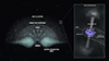 |
Fig. 1. Scheme of the proposed scenario (not to scale). The wind ejected from the accretion disk of the SMBH interacts with the BHs forming the cluster. Because of the combination of the velocities of the SMBH wind (vw) and the orbital motion of the BH (vBH), a bow shock forms in the direction of the relative velocity (vrel). The dense wind is captured by the BH via cylindrical accretion. A small accretion disk forms around the BH and jets are produced with two assumed shock-prone zones (recollimation and terminal regions). |
Accretion onto isolated stellar BHs has been studied by Tsuna et al. (2018) and Ivanov et al. (2019). In particular, Maccarone (2005), Fender et al. (2013), and Tsuna & Kawanaka (2019) showed that these BHs can be detected, and Barkov et al. (2012) demonstrated that jets can be produced despite the very low accretion rates involved. On the other hand, observable signatures of stellar mass BHs embedded in SMBH disks have recently been studied by Tagawa et al. (2023a,b), and Rodríguez-Ramírez et al. (2024).
In this paper, we explore the possibility of detecting electromagnetic signatures from a cluster of BHs orbiting a super-Eddington SMBH without jets, as in the case of some Seyfert 1 galaxies. We consider an SMBH in the super-Eddington regime (either a persistent regime or a transient regime generated by a TDE) that ejects winds, and we characterize the accretion of the dense wind onto the stellar BHs and the subsequent formation of jets. We calculate the thermal emission from the disk, the nonthermal emission from the inner jet, and the thermal and nonthermal radiation from the terminal regions of the jet. We then correct the emission for absorption locally and in the wind photosphere. Finally, we consider whether the integrated spectral energy distribution (SED) shows any features that could reveal the presence of a BH cluster at the center of some galaxies.
The paper is organized as follows. We begin by characterizing the astrophysical scenario in which stellar BHs orbit the SMBH, decribing its disk and wind, the population of BHs, and the accretion of an isolated BH moving in a dense wind (Sect. 2). In Sect. 3 we study the production of jets in BHs and their interaction with the SMBH wind. We then describe the associated radiative processes and the absorption of the radiation. The results are presented in Sect. 4, and after a discussion (Sect. 5), we conclude.
2. Model
We assumed that the BHs from the cluster have typical masses of MBH ∼ 10 M⊙ (Miralda-Escudé & Gould 2000; McKernan et al. 2011) and orbit a superaccreting nonjetted SMBH of MSMBH = 107 M⊙ in circular and Keplerian orbits. The stellar BHs accrete matter from the dense wind ejected from the accretion disk of the SMBH. The accretion onto the BHs proceeds via the BHL regime, and jets are generated by magneto-centrifugal effects (e.g., Spruit & Uzdensky 2005). Fig. 1 shows a scheme of this scenario. In what follows, we first describe the SMBH and its wind, then the cluster of BHs orbiting the central SMBH, and finally, the accretion onto the BHs, considering three different scenarios. Table 1 summarizes the values of the main parameters of the system.
Basic parameters of the SMBH, BHs, and cluster.
2.1. Accretion disk of the SMBH and its wind
We neglected the self-gravity of the disk of the SMBH, which is under a super-Eddington accretion regime in the outer part of the disk,  , where Ṁinput is the supply of mass per unit time. We explored three super-Eddington regimes with rates of ζ = 10, 102, and 103. The Eddington rate is given by

where LEdd is the Eddington luminosity (defined as the luminosity required to balance the gravitational attraction of the accreting object by radiation pressure), η ≈ 0.1 is the accretion efficiency, M is the accretor mass in units of solar mass, and c is the speed of light.
In the cases of high accretion rates (ζ ≳ 102), we assumed that the super-Eddington regime of the SMBH is caused by the disruption of a star in a TDE. During a TDE, the peak mass fallback rate is given by (Stone & Metzger 2016)
with M* the mass and R* the radius of the disrupted star. This super-Eddington phase remains for a timescale
The central parsecs of galaxies are expected to harbor early massive stars, which means that when we calculate the accretion peak for an O5 star with mass 37 M⊙ and radius 11 R⊙ (Kobulnicky et al. 2019), for example, we obtain  , a superaccretion regime that lasts for a time tEdd ≈ 7 yr.
The critical radius of the disk, given by rcrit ∼ 40 ζ rg, SMBH, corresponds to the distance from the SMBH at which the outer standard disk (Shakura & Sunyaev 1973) changes to the radiation-dominated inner disk (Fukue 2004). Here, rg, SMBH = GMSMBH/c2 is the gravitational radius of the SMBH, with G the gravitational constant. The disk becomes geometrically thick in the inner region, where the ejection of winds by the radiation force helps to regulate the mass accretion rate onto the SMBH (Ṁacc) at the Eddington rate1. This regulation results in a total mass-loss rate Ṁw that is approximately equal to the accretion input,  .
.
We assumed that the wind ejected from the SMBH disk is smooth and expands isotropically at a constant velocity, estimated to be  (King 2010). Since βw ≪ 1 for ζ ≫ 1, the Lorentz factor of the wind is γw ≈ 1, and therefore, the wind properties do not depend on the line of sight (Θ), so that 1 − βwcosΘ ≈ 1 (see e.g., Abaroa & Romero 2024). The density of this wind at a distance r from the BH is
We assumed steady state, so that vw and Ṁw are constant, and therefore, the density only depends on the distance to the SMBH.
The wind itself is opaque until it reaches the photospheric radius, where it becomes transparent to its own radiation. The apparent photosphere is defined as the surface where the optical depth τphoto is unity for an observer at infinity. Its location zphoto, measured from the equatorial plane, can be found by integrating over the wind density (Fukue 2009),

where κco ≈ κ is the opacity and ρco ≈ ρw (the subindex co refers to the comoving frame). Since we assumed a fully ionized wind, the opacity is dominated by free electron scattering (κ = σT/mp, where σT is the Thomson scattering, and mp is the proton mass). The location of the wind photosphere is completely determined by the mass-loss rate and thus by the accretion input of matter. The apparent photosphere of this wind is of interest for the calculation of the absorption of the radiation.
Since the wind is optically thick, we assumed that it radiates as a blackbody. The temperature measured by an observer at infinity is given by (Fukue 2009)
where ė = 0.1 is the fraction of LEdd that passes the comoving luminosity of the wind (Sotomayor & Romero 2022). The radiative power of the wind in supercritical sources is then limited to the Eddington luminosity (Zhou et al. 2019). The numerical results of the photospheric temperature and height for the three scenarios are detailed in Table 2.
Parameters of the three scenarios we modeled for the accretion rate onto the SMBH.
This wind ejected by the accretion disk interacts with the BHs orbiting the SMBH, but before studying this interaction, we present a description of the BH population in the next subsection.
2.2. Cluster of BHs
The SMBH dominates the orbital evolution of the objects within an influence radius given by (Kormendy & Ho 2013)
where σ*2 is the dispersion of the velocities of the orbital objects (Peebles 1972), and it is calculated from the relation (Gondán & Kocsis 2022)

In our case, σ* = 9.14 × 106 cm s−1, so that rcluster ≈ 1.65 × 1019 cm ≈ 5.48 pc ≈ 107 rg, SMBH.
Most of the mass contained within this radius corresponds to stars and BHs. Each population is associated with a radial function of density, ρ*(r) and ρBH(r), where r is the distance to the SMBH. The density profile of BHs is a fraction C = (0.23 M⊙/MBH)1/2 of the stellar profile (Miralda-Escudé & Gould 2000)2,
The cumulative mass distribution in a sphere with a radius r is obtained by integrating 4πr2ρBH(r), which gives
so the number of BHs inside the sphere is estimated to be NBH(r)∼mBH(r)/MBH. We obtain a total number of NBH ∼ 1.5 × 10⁵ isolated BHs that form the cluster for the assumed BH masses3. Figure 2 shows the distribution of BHs within the radius of the cluster projected on the rz-plane, where each dot represents an individual BH.
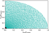 |
Fig. 2. Distribution of BHs within the cluster projected on the rz-plane, where each dot represents a BH of 10 M⊙. Both axes are on a linear scale and represent the distance rorb to the SMBH in units of the cluster radius. The SMBH (large black dot, not to scale) yields (0, 0). |
2.3. Accretion onto stellar black holes
Stellar BHs orbiting the SMBH capture matter from the dense wind ejected by its accretion disk. Since the relation between the velocities of the wind and the BHs is not negligible, the accretion is not spherical, but cylindrical. That is, small accretion disks with radii RHL = 2GMBH/vrel2 are formed around the BHs via the BHL regime (see section 4.3 of Romero & Vila 2014, for a full description of this regime). In the latter expression, vrel2 = vw2 + vBH2 is the composition of the velocities of the spherical wind ejected from the SMBH disk and the BH in its orbital motion, vBH2 = GMSMBH/rorb. We assumed that the distance between the SMBH and the BH is constant, r = rorb (circular Keplerian orbits). The outer radii of the accretion disks are in the range RHL ∼ 104 − 5 rg, BH for BHs at different distances.
The accretion disk is formed when the circularization radius (Rcirc) is larger than the radius of the innermost stable circular orbit of the BH (RISCO = 6 rg, BH, for a nonrotating BH). The former is given by Rcirc = J2/GMBH, where J = RHL vrel is the angular momentum per unit mass of the wind when it is trapped in the gravitational field of the BH. We then have Rcirc = RHL2 vrel2/G MBH = 4G2MBH2 vrel2/G MBH vrel4 = 4 G MBH/vrel2. Hence, Rcirc ≈ 4 × 1027 cm3 s−2/vrel2 for the assumed value of the BH mass, which is greater than RISCO ∼ 9 × 106 cm if vrel < 0.7 c (this condition is always satisfied in this work).
The accretion rate of a BH by the BHL mechanism reads
Replacing the expressions for ρw (Eq. (4)) and vrel into the above equation, we obtain

The accretion disk of the SMBH is regulated at the Eddington rate, so that the mass-loss rate must be approximately equal to the accretion rate,  . Since the SMBH is supercritical,
  , with ζ ≫ 1, where the Eddington rate is given by Eq. (1). Then, the accretion rate of the BH (with all quantities in cgs units) is
![$$ \begin{aligned} \dot{M}_{\rm BH}\approx 3.135\times 10^{-30} \cdot \frac{\zeta \, M^2_{\rm BH} \, M_{\rm SMBH} }{r^2_{\rm orb} v_{\rm w}(v^2_{\rm w}+v^2_{\rm BH})^{3/2}} \ [\mathrm{g\,s^{-1}}]. \end{aligned} $$](/articles/aa/full_html/2024/11/aa51903-24/aa51903-24-eq29.gif)
The accretion rate onto the isolated BHs thus depends on four parameters: the superaccretion factor of the SMBH (ζ), the BH masses (MBH and MSMBH), and the location of the BHs (rorb). Therefore, when we fix the masses and the superaccretion factor, the accretion of matter onto the BHs only depends on the orbital radius. The accretion disk around the BH forms on the orbital plane, where the initial direction of the accreting material depends on the relation between the orbital velocity and the wind velocity. Figure 3 shows the accretion rate of stellar BHs on a logarithmic scale in units of the BH Eddington rate as a function of the orbital radius (in units of the gravitational radius of the SMBH) for the three different accretion rates onto the SMBH (ζ1 − ζ3: yellow, green, and light blue curves in the plot).
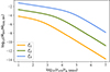 |
Fig. 3. Accretion rates onto the isolated BHs orbiting the SMBH in units of their Eddington rate (see Eq. (13)) as a function of their distance from the center of the galaxy. Both axes are on a logarithmic scale. We plot the three regimes of SMBH accretion (ζ1 − ζ3 from bottom to top). |
We studied BHs inside (rorb ≤ zphoto) and outside the photosphere (rorb > zphoto). We note that in the case of scenario ζ1, almost the entire population of BHs is outside the photosphere. We computed the emission from the accretion disks only for the BHs outside the wind photosphere. In most cases, the accretion proceeds in the low-accretion ADAF (advection-dominated accretion flow) regime, with  . Since the disk contribution is small in any case, we assumed for simplicity that the disks radiate in the standard regime of Shakura & Sunyaev (1973). This contribution should therefore be considered only as an upper limit.
3. Jet
The BHs with their small accretion disks generate two jets that propagate in opposite directions through the wind of the supercritical SMBH (see Bosch-Ramon & Barkov 2016). In this section, we first characterize the jet and its launch and then study the shocks at the base (recollimation) and the lobes (terminal region). We then discuss particle acceleration, cooling, and transport. Table 3 lists the values for the parameters of BHs near the wind photosphere for the three scenarios we considered.
Parameters of BHs and their jets.
3.1. Launch and general properties
We assumed that the jet is perpendicular to the plane of the accretion disk and is fully formed at a distance of z0 = 100 rg from the BH, with an initial radius of r0 = 0.1 z0 = 10 rg. Afterward, the outflow expands as a cone with radius rj(z) = r0(z/z0) = 0.05 z (i.e., with a semi-opening angle of θj ≈ 3°, see e.g. Pepe et al. 2015). According to the disk-jet coupling hypothesis of Falcke & Biermann (1995), the kinetic power of each jet is assumed to be proportional to the accretion power, Lj = qjLaccr, where qj = 0.1 is a moderate efficiency in transferring power from the disk to the jet, and  . A fraction qrel ≈ 0.1 of the jet power is expected to be in the form of relativistic particles. Then we can write Lrel = qrel Lj. We included both the hadronic and leptonic fractions, Lrel = Lp + Le.
We considered two acceleration regions mediated by shocks for relativistic particles in the jet: one near its base (recollimation), and the other at the terminal region (lobes)4. The energy distribution between hadrons and leptons is unknown; we assumed an equipartition near the base of the jet (Lp = Le) and a hadronic-dominated scenario in the terminal region (Lp = 100 Le) (for a discussion about this assumption see e.g., Romero & Vila 2008; Bordas et al. 2009). We describe these regions in the following two subsections.
3.2. Recollimation
The recollimation of the jet produced by the wind of the SMBH determines the location of the acceleration region near the base of the jet. Given the orbital radii at which the BHs are located, we assumed that the fluid streamlines are parallel when the wind reaches the BHs.
The ram pressure of the wind at a height z above the BH is
where we considered the approximation rorb ≫ z. On the other hand, the jet lateral pressure is (Yoon & Heinz 2015; Bosch-Ramon & Barkov 2016)
where vj is the bulk velocity of the flow. We assumed a moderate value for the Lorentz factor γj = (1 − vj2/c2)−1/2 = 3, so vj = 0.943 c (Heinz & Sunyaev 2002). We can find the height zrecoll of a recollimation shock in the jet by equaling these pressures, Pram, j = Pram, w,
![$$ \begin{aligned} z_{\rm recoll}=[4L_{\rm j}\beta _{\rm j}v_{\rm w}r_{\rm orb}^2 / \gamma _{\rm j}(\gamma _{\rm j}-1)c \dot{M}_{\rm w}v_{\rm rel}^2]^{1/2}. \end{aligned} $$](/articles/aa/full_html/2024/11/aa51903-24/aa51903-24-eq39.gif)
The magnetic field at the base of the jet, B0 = B(z0), can be estimated from the equipartition between the magnetic and kinetic energy densities at z0 (ϵB = ϵK), where the Alfvén radius is (rA ≡ z0) and the geometry of B starts to change from poloidal to toroidal, B02/8π = Lj/2πr02vj. The magnetic field in the jet decreases with distance z from the BH: when the flow expands adiabatically, B(z) = B0(z0/z)m, where m is the magnetic exponent which depends on the geometry of B. In our case, m = 1 because the magnetic field has a toroidal geometry for z > z0.
On the other hand, the number density of cold protons at a distance z from the BH in the jet is  , where the mass-loss rate in the jet is given by
  .
.
3.3. Terminal jet
The head of the jet propagates through the wind. Its length lj at a time t is given by (Kaiser & Alexander 1997):
We assumed that the lifetime of the single microquasar lasts for a fraction of the time that the SMBH spends in the super-Eddington regime (see Eq. (3)). We adopted conservative ages of 15, 5, and 1 yr for scenarios ζ1, ζ2, and ζ3, respectively. The jet lengths were about lj ∼ 1014 cm for all scenarios and orbital distances (the larger the orbital distance, the longer the jet). The jet length always exceeds the recollimation height, lj ≫ zrecoll (see Table 3).
At the head of the jet, two shocks are generated: a forward radiative shock that propagates into the wind, and a reverse adiabatic shock that propagates into the jet. The radius of the bow shock is assumed to be ∼lj/3 (Bordas et al. 2009). Particle acceleration to relativistic energies only occurs in the reverse adiabatic shock (see characterization of these shocks in Abaroa et al. 2023). Conversely, in radiative shocks, the gas emits thermal optically thin radiation, and no particle acceleration is produced (see e.g. Longair 2011). We assumed a magnetic field of B ≈ 10 μG for this region, which corresponds to that of the compressed medium (the magnetic field can take maximum values of ∼100 μG in these scenarios, see Araudo et al. 2015, 2016). The proton number density is np = ρw/mp.
3.4. Relativistic particle acceleration, cooling, and transport
The acceleration rate for a charged particle in a magnetic field B through first-order Fermi mechanism is given by  , where E is the energy of the particle, and ηacc is a parameter characterizing the efficiency of the acceleration mechanism (we assumed a mildly efficient acceleration in all regions, ηacc = 0.1).
Particles accelerated at the shocks can cool by various processes and produce thermal and nonthermal radiation. The timescales associated with this cooling are related to the total energy loss of the particles: dE/dt ≈ −E/tcool, where the total cooling rate is  (ti corresponds to each timescale of the cooling processes involved).
We assumed advective escape at the base of the jet and diffusive escape at the lobes. When the cooling timescales are shorter than the escape timescales, particles radiate before escaping from the acceleration regions. The maximum energy for each type of particle can be derived by equating the acceleration rate to the total cooling or escape rate. This energy cannot exceed the maximum energy imposed by the Hillas criterion.
Radiative cooling is caused by nonthermal processes as a consequence of the interaction of particles with ambient fields and matter.
Our model is lepto-hadronic, and we therefore numerically calculate the following cooling processes:
– Synchrotron: Interaction of protons and electrons with the ambient magnetic field.
– Inverse Compton: Collision of relativistic electrons with photons of the ambient radiation field.
– Self-synchrotron Compton (SSC): Collision of relativistic electrons with photons of the synchrotron radiation field.
– Relativistic Bremsstrahlung: Coulombian interactions between relativistic electrons and cold matter.
– Thermal Bremsstrahlung: Free-free radiation by Coulombian interactions.
– Photo-hadronic interactions: Interaction of highly relativistic protons with photons of the surrounding radiation field. This interaction produces pions that decay into gamma rays, e+e− pairs, and neutrinos.
– Proton-proton: Collision of relativistic protons with cold matter. This process is also a source of gamma rays, pairs, and neutrinos.
The relativistic particles have a distribution given by dN = n(r, E, t)dEdV, where n is the particle number density, t is the time, r is the position, V is the volume, and E is the energy. The transport equation governs the evolution of this distribution (Ginzburg & Syrovatskii 1964). We solved this equation numerically in steady state and in the one-zone approximation and assumed an injection spectral index for the particles of p ∼ 2 in all cases (e.g., Drury 1983; Romero & Vila 2008; Pepe et al. 2015).
After we determined the relevant processes involved in the cooling and calculated the particle distributions, we calculated the SED of the radiation produced by the particles as they interact with the magnetic, matter, and radiation fields (we refer to Romero & Vila (2008, 2014) and references therein for additional details on nonthermal processes and to Longair (2011) for details on thermal Bremsstrahlung (see Chapter 6.5)).
4. Results
The results for the accretion onto the BHs and their location in the cluster (along with the properties of the supercritical SMBH wind) were presented in Sect. 2. In this section, we focus on the results for the radiation produced by the system.
As mentioned in Sect. 2.2, we applied our model to a population of ∼1.5 × 10⁵ BHs with typical masses of 10 M⊙ orbiting a 107 M⊙ SMBH. The SED of the entire population of BHs was estimated as follows. First, we calculated the luminosity of individual BHs at different orbital radii BH(i), with accretion rates according to the results shown in Fig. 3. The total radiative contribution LBH(i) of a single microquasar corresponds to the thermal emission from its mini-disk (Ldisk), the nonthermal emission from the recollimation shock (Lrecoll), the nonthermal emission from the reverse shock of its jet (Llobe, NT), and the thermal emission from the forward shock in the lobes (Llobe, thermal): LBH(i)(Eγ) = Ldisk(i)(Eγ)+Lrecoll(i)(Eγ)+Llobe, NT(i)(Eγ)+Llobe, thermal(i)(Eγ). The emission produced at the recollimation shock was calculated taking relativistic effects into account: We calculated the Doppler boost factor D2 = (γj − βjcosαj)−1, and we then average the emission over αj from 0° to 90°. When L′recoll(Eγ) is the comoving emission, then the boost luminosity in the observer’s frame is  L′recoll(Eγ) (Lind & Blandford 1985).
The second step was to calculate the gamma absorption by pair creation from photon-photon annihilation. We considered two radiation fields: the synchrotron emission produced in the jet (a), and photons of the ambient radiation field produced by the wind photosphere (b). Since the wind is dense, we also calculated the absorption by Thomson scattering (c) for the BHs inside the photosphere. The attenuation factor is given by e−τ(Eγ), where τ = τa + τb + τc is the optical depth of the medium, which quantifies the absorption of radiation by all the processes involved. The attenuated luminosity is then LBH(i)′(Eγ) = LBH(i)(Eγ)⋅e−τ(Eγ).
Finally, we set up spherical shells centered on the SMBH for the different orbital radii considered so far, calculated the number NBH(i) of BHs contained therein, and estimated the luminosity of the shell, assuming that all BHs produce approximately the same radiation (the shell is thin enough to guarantee homogeneity conditions): Lshell(i)(Eγ) = NBH(i) LBH(i)(Eγ). The total SED of the cluster is the sum of all contributions, Ltotal(Eγ) = ∑iLshell(i)(Eγ).
In what follows, we first detail the results for the emission from one single microquasar, and we then present the results for the emission from the entire population of BHs, plus the thermal contribution from the wind photosphere.
4.1. Emission from individual sources
All the thermal and nonthermal processes ultimately depend on the accretion rate onto the BHs and thus on the distance to the SMBH. A higher accretion rate provides more energy to transfer power to the jet, so that the major radiative contributions are produced by the BHs that are located just above the photosphere of the SMBH wind, rorb ≳ zphoto. The length of the jet is also a crucial parameter for the thermal emission of the lobes.
The emission of BHs inside the photosphere is entirely suppressed for photon energies ≲1 MeV, except for those close to the photosphere border, whose emission is partially attenuated and provides the radiation that can escape from inside the photosphere and dominates the emission for that group of BHs. Below, we describe the results we obtained for the different parts of the single microquasar for the three scenarios we considered. In scenario ζ1 almost the whole population of BHs is outside the photosphere and we therefore did not calculate the contribution from the inner BHs, while in scenarios ζ2 and ζ3, we ruled out the thermal emission produced inside the photosphere because it is totally suppressed. Since the outer radii of the accretion disks are limited by the BHL radius, their spectra resemble a blackbody and not a characteristic multicolor disk.
In what follows, we describe the radiative output for the different emission regions of the individual sources in the three scenarios (Fig. 4 shows the results for the entire population described in the next subsection, not for the individual sources).
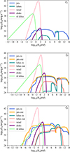 |
Fig. 4. Emission of the entire system for scenarios ζ1, ζ2, and ζ3, from top to bottom. We plot the nonthermal SEDs of the base (jets) and terminal jets (lobes) for two groups of BHs, those inside (in) and outside (out) the photosphere (except for the case ζ1, where we present only the results for BHs outside the photosphere). We also plot the SEDs of the SMBH wind photosphere, the accretion disks of the BHs, and the thermal lobes (th lobes) outside the photosphere. |
Scenario ζ1:
– Accretion disks: The emission peaks at ultraviolet (UV) energies for the BHs near the photosphere and at optical energies for those in the outer cluster. The luminosity range is ∼1025 − 33 erg s−1, where the disks with a maximum in the UV are more powerful.
– Recollimation shock: The recollimation height is ∼108 cm for the BHs that lie close to the photosphere. The magnetic field there is ∼105 G, and the dominant cooling process for accelerated electrons is synchrotron in all cases, reaching maximum energies of 1011 eV. The advective escape dominates in all cases for protons, reaching energies in the range 1014 − 1015 eV. The emission is completely dominated by the BHs that lie close to the photosphere, producing synchrotron radiation with a luminosity ∼1031 erg s−1 in the range 10−1 − 107 eV, and π0-decay gamma emission due to pp interaction with a luminosity above ∼1030 erg s−1 in the range 108 − 1012 eV.
– Nonthermal lobe: Electrons mainly cool by IC and Bremsstrahlung, reaching energies in the range 108 − 1011 eV. Protons reach their maximum energy of 1012 eV in the lobes of BHs just above the photosphere, with pp being the dominant cooling mechanism. The SEDs of the BHs are dominated by the IC and pp emission, with luminosities for the BHs near the photosphere of ∼1030 and ∼1032 erg s−1, respectively. Photon-photon annihilation is irrelevant.
– Thermal lobe: The emission is completely dominated by the BHs near the photosphere, with a maximum luminosity of ∼1039 erg s−1 at 10−2 eV. This is the dominant emission mechanism for scenario ζ1.
Scenario ζ2:
– Accretion disks: The emission peaks at soft X-ray energies for the BHs near the photosphere and at UV energies for those in the outer cluster. The luminosity range is ∼1028 − 34 erg s−1, where the disks with a maximum at X-rays are more powerful.
– Recollimation shock: The recollimation height is in the range ∼109 − 1011 cm above the BHs. The magnetic field there for the BHs outside the photosphere is ∼10 − 104G, and the dominant cooling process for the accelerated electrons is synchrotron in all cases, reaching energies in the range 1011 eV (near the photosphere) and 1013 eV (near the cluster radius). The advective escape dominates in all cases for protons reaching energies in the range 1012 − 1015 eV. The emission is completely dominated by the BHs that lie close to the photosphere, producing synchrotron radiation with a luminosity ∼1031 erg s−1 in the range ∼10−2 − 107 eV, and π0-decay gamma emission due to pp interaction with a luminosity ∼1030 erg s−1 in the range 108 − 1012 eV. Internal and Thomson absorption is almost total for the BHs inside the photosphere and is not relevant for those outside it.
– Nonthermal lobe: Electrons mainly cool by IC and Bremsstrahlung, reaching energies in the range 109 − 1012 eV. The maximum energy of the protons is 1012 eV; diffusive escape dominates in all cases, with pp being the dominant cooling mechanism. The SEDs of the BHs outside the photosphere are dominated by IC and pp emission, with luminosities of ∼1030 and ∼1032 erg s−1 for the BHs outside but close to the photosphere. Photon-photon annihilation is only relevant for BHs inside the photosphere.
– Thermal lobe: The luminosity range is ∼1026 − 1037 erg s−1, and in all cases, the emission peaks at 1 eV. This is the dominant emission mechanism for scenario ζ2.
Scenario ζ3:
– Accretion disks: The emission peaks at soft X-ray energies for the BHs near the photosphere and at UV energies for those in the outer cluster. The luminosity range is ∼1031 − 34 erg s−1, where the disks with a maximum in X-rays are more powerful. This is the dominant emission mechanism for scenario ζ3.
– Recollimation shock: The recollimation height is in most cases ∼1011 cm above the BHs. The magnetic field there for the BHs outside the photosphere ranges from ∼10 − 100 G and the dominant cooling process for the accelerated electrons is synchrotron in all cases, reaching energies in the range of 1010 eV (near the photosphere) and 1013 eV (near the cluster radius). The advective escape dominates in all cases for protons, reaching energies in the range 1014 − 1015 eV. Again, the emission is completely dominated by the BHs that lie close to the photosphere, producing synchrotron radiation with a luminosity above ∼1031 erg s−1 in the range 10−3 − 105 eV, and π0-decay gamma emission due to pp interaction with a luminosity above ∼1030 erg s−1 in the range 108 − 1012 eV. As in the case of ζ2, internal and Thomson absorption is almost total for the BHs inside the photosphere and negligible for those outside.
– Nonthermal lobe: Electrons mainly cool by IC and Bremsstrahlung, reaching energies in the range 109 − 1011 eV. Protons reach their maximum energy of 1011 eV in the lobes of the BHs just above the photosphere, while the pp interaction suppresses the acceleration for those close to the SMBH. Diffusive escape dominates in all cases, with pp being the dominant cooling mechanism. The SEDs of the BHs outside the photosphere are dominated by the IC and pp emission, with luminosities of ∼1030 and ∼1032 erg s−1 for the BHs near the photosphere. Photon-photon annihilation is only relevant for the BHs inside the photosphere.
– Thermal lobe: Although all thermal lobes are about the same size, the spectrum is more luminous for the BHs that lie close to the photosphere because the density of the medium is higher. The luminosity ranges from ∼1028 − 1033 erg s−1, and in all cases, the emission peaks at 10 eV.
4.2. Emission from the entire system
Figure 4 shows the thermal and nonthermal radiative contributions of the whole system for scenarios ζ1, ζ2, and ζ3 (from top to bottom). We separated the nonthermal emission into two groups: the BHs inside and outside the photosphere of the SMBH wind (except for case ζ1, where we present only the results for the BHs outside the photosphere). The wind produces the peak contribution in all scenarios, with luminosities ∼1042 − 1044 erg s−1 in the infrared. The thermal emission from the lobes of the jets is the dominant radiation produced by the clusters of scenarios ζ1 and ζ2. Conversely, in the ζ3 scenario, the dominant emission of the cluster is in the X-ray band and is mainly produced by the electron synchrotron mechanism at the base of the jets outside the photosphere, reaching a luminosity of ∼1036 erg s−1 for the entire population of BHs. The accretion disks also contribute at very soft X-rays with ∼1037 erg s−1.
The very high energy emission is dominated by the π0-decay due to the pp interaction at the base and the lobes. The emission from the base of the jet dominates that from its terminal region in all cases and energies, except for the 108 − 1010 eV energy range, where the luminosity caused by pp interactions from the lobes is slightly dominant.
Figure 5 shows the total SEDs of the three scenarios and the sensitivities of different space- and ground-based telescopes for a distance of 3 Mpc corresponding to a nearby galaxy. In scenarios ζ1 and ζ2, the emission from a BHs cluster in a nearby galaxy is potentially detectable only at energies in the range 10−7 − 10−4 eV by the ground-based instruments Atacama Large Millimeter Array (ALMA), Very Large Array (VLA), next-generation VLA (ngVLA), and Square Kilometer Array (SKA1 and SKA2), although in the case of ALMA, the emission would probably be difficult to separate from that coming from the SMBH wind. In scenario ζ3, the electron synchrotron emission at such low energies could only be detected by ngVLA or SKA2. In the X-ray band, the XMM-Newton and Chandra telescopes might both also detect the synchrotron emission of the recollimation shock (although the detection margin is narrow with the parameters assumed in our model), while the NuStar telescope is not able to detect the emission in any case.
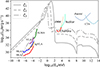 |
Fig. 5. Total SEDs of the three scenarios and sensitivity curves of several ground- and space-based telescopes, assuming a distance to the source of ∼3 Mpc. We plot with solid, dashed, and dot-dashed lines the total SEDs of scenarios ζ1, ζ2, and ζ3. The sensitivities of ALMA, VLA, and ngVLA are adapted from Guo et al. (2020) (1 h on-source integration); the SKA1 and SKA2 sensitivities are taken from Wang et al. (2024) (1 h); the sensitivities of XMM-Newton (105 s), Chandra (105 s), NuStar (106 s), Fermi (10 yr), and CTA (50 h) are taken from Lucchetta et al. (2022) and references therein (the integration time for observations is given in brackets). |
The gamma-ray emission predicted by our model is not detectable by any of the current instruments, whether ground-based like Cherenkov Telescope Array (CTA) or space-based like Fermi.
5. Discussion
5.1. Dependence of the emission on the parameters
In all scenarios and for all emission regions in the single microquasars, the radiative output is strongly dominated by the BHs near the photosphere. The size of the latter depends on the accretion rate onto the SMBH (the higher the rate, the larger the photosphere). The emission from a small number of BHs in the central parsec then dominates the remaining population within the gravitational influence radius rcluster. We note that the dense medium in which the BHs orbit can induce a migration to closer orbits over long periods of time, so that perhaps the population of BHs near the photosphere is underestimated in our model, and therefore, the emission is higher than predicted.
We have applied our model to conservative values for the BH masses: MSMBH = 107 M⊙ and MBH = 10 M⊙. Since  , then
  (see Eq. (13)), and thus, a lower SMBH mass leads to a higher accretion rate onto the BHs. In addition, for the BHs we have
  , so that when we consider MBH = 30 M⊙ and MSMBH = 106 M⊙, then ṀBH increases by an order of magnitude. The accretion onto BHs is even more accentuated in the case of dwarf galaxies with MSMBH ∼ 105 M⊙ (see e.g. Baldassare et al. 2015). Since
  and the radiative output of the system is ∝Lj, the luminosity of the cluster can increase up to two orders of magnitude in a galactic center with these masses. The accretion rate onto the stellar BHs is also strongly sensitive to the velocity of the SMBH wind, since
  . When instead of a smoothed outflowing wind, we consider inhomogeneities or retarding effects due to internal interactions, then its velocity may decrease (Shore 1992). For example, reducing the wind speed by half would increase the accretion ṀBH by a factor of 10.
We did not consider the possible rotation of the BHs. For spinning BHs, the disk-jet coupling factor qj can be larger than 0.1, leading to more powerful jets (Tchekhovskoy et al. 2011; McKinney et al. 2012). Furthermore, the innermost stable circular orbit may be smaller than 6 rg, BH (reaching 1 rg, BH for maximally rotating BHs), so that the thermal emission from the disks will have its maximum at higher energies, favoring detection by X-ray telescopes in scenario ζ3. We note, however, that the Blandford–Znajek mechanism can be activated in spinning BHs under certain circumstances, producing jets without the formation of an accretion disk, as shown by Barkov & Khangulyan (2012). A harder spectral index for the injection of particles at the base of the jet would also increase the X-ray luminosity. On the other hand, a lower Lorentz factor of the jet would lead to stronger emission from the recollimation shock in the observer’s frame, which could be higher by up to an order of magnitude.
5.2. Detectability
The rate of TDEs is theoretically estimated to be 10−4 yr−1gx−1 (Stone & Metzger 2016), although other authors suggested higher rates, from 10−3 yr−1gx−1 (Kaur & Stone 2024) to 10−2 yr−1gx−1 (Tadhunter et al. 2017). These theoretical predictions differ from observations, the rate of which is ∼10−5 yr−1gx−1. Stone & Metzger (2016) stated that selection effects, small number statistics, and the possible influence of dust or photoelectric extinction could all contribute to this discrepancy between theory and observations (TDEs are difficult to observe because they have their characteristic emission at optical frequencies, and the galactic centers are heavily obscured by dust).
In transient events, jet lengths are strongly constrained. Instead, a persistent super-Eddington scenario with typical microquasar ages of 105yr leads to jet lengths on the order of 0.1 − 1pc. In this case, the terminal lobes of the jet (both the reverse- and forward-shock regions) will be much larger, since the size of the lobes is proportional to the length of the jet, so that the emission regions and luminosity will be larger as well. The thermal emission in cases ζ1 and ζ2 would be higher, and a larger acceleration region of the reverse shock in scenario ζ3 will also allow the particles to cool by the synchrotron mechanism, favoring radio emission in the SKA range.
The least likely scenario to be detected is ζ3 because of the very high accretion rate and the duration of the TDE in this case. Its detection should occur in the X-ray band and could only happen for nearby galaxies. Conversely, BHs of scenarios ζ1 and ζ2 could be detected at very low energies with the ngVLA and SKA telescopes from a distance up to 100 Mpc in the case of SKA1 and SKA2.
The emission from X-ray binaries orbiting the SMBH would probably exceed the cluster emission in the X-ray band. When we compare our results with Cyg X-1 (see Pepe et al. 2015), for example, the emission from isolated BHs dominates in the radio bands by many orders of magnitude.
5.3. Further considerations
The effect of the strong wind on the jet can lead to jet-bending effects, as detailed, for example, by Yoon & Heinz (2015) and Yoon et al. (2016) for the case of X-ray binaries. Bosch-Ramon & Barkov (2016) also investigated orbital effects on the jet, such as the Coriolis effect, which in certain cases can lead to a helical structure of the jet trajectory (see also Bosch-Ramon & Bellomo 2020). We neglected these effects in this work, although they may be relevant for some of the BHs in the cluster under certain conditions, especially the bending (the Coriolis force affects the system on scales much larger than the jet lengths discussed in this paper).
In a TDE, the wind is produced during the super-Eddington phase. The duration of this stage in the scenario ζ3 is estimated to be ∼1 yr, and the wind has a velocity of ∼108 cm s−1. Since the BHs that contribute most to the radiation are located at ∼4 × 1017 cm, just above the wind photosphere, it takes ∼30 yr for the wind to reach these BHs, which is much longer than the super-Eddington phase. In these cases, the outflow from the SMBH resembles a dense shell illuminating the single BHs from the cluster at different times (first those closer to the SMBH, then those farther away). Therefore, there could be a delay of years between the emission of the TDE from the core of the system and the radiative activation of the BHs.
After the tidal disruption of the star, the wind launched by the transient accretion disk formed around the SMBH propagates as an expanding shell with a constant thickness δx, so that at some point it becomes transparent to the inner radiation. This can be roughly estimated by imposing τ = σT δx n(d)≲1, where τ is the optical depth, σT is the Thomson cross-section, and n is the number density of the wind at a certain distance d from the SMBH. For example, for the parameter values in the scenario ζ3, the super-Eddington phase lasts t ∼ 1 yr, and the thickness of the wind shell therefore is vw t ∼ 1015 cm. At an orbital radius zphoto, ζ3/2 ∼ 1017 cm (see Table 2), the ambient number density is ∼3 × 108 cm−3, so that τ < 1 and the inner radiation passes through the wind. The implications of this situation will be addressed in future work.
In TDEs, the emission from the AGN is produced during the lifetime of the disk. First, the accretion disk forms, producing a multiband spectrum. Some time later, the winds are launched and screen the emission from the disk. Radio emission could be present when the system has a jet, but we assumed a nonjetted SMBH (Stone & Metzger 2016, suggesting that only a fraction of 0.3 percent of TDEs produce jets). In addition, jet activity is significantly shorter than the lifetime of the accretion disk formed during a TDE (e.g., Mimica et al. 2015; Zubovas 2019). Furthermore, if there is a delay between the TDE emission and the illumination of the individual BHs in the cluster, as we suggested above, the transient active galaxy turns off as the BHs turn on. This could also aid in the detection of the BHs because the primary event will alert us to the possibility that the mechanisms discussed in this paper are activated.
The terminal region of the jets injects cosmic rays with energies up to ∼1 TeV. The relativistic protons and electrons escaping from the lobes interact with the surrounding medium, producing diffuse emission in the surroundings through pp and Bremsstrahlung interactions. In addition, when protons escape from the central region, they may interact with cold matter at larger distances, producing gamma rays. Neutrons created at the recollimation shock via p + γ → n + π can escape from the jet and interact with the dense surrounding gas, also leading to the production of gamma rays (Escobar et al. 2021).
The jets of the stellar BHs orbiting close to the SMBH can also interact with the super-Eddington disk. This interaction can lead to particle acceleration, nonthermal emission, and neutrinos under certain conditions. Neutrino emission can play some role in the detection of these systems, since the wind photosphere is transparent to them. The interaction of jets with dense targets of matter was addressed, for example, by Romero & Orellana (2005), who studied misaligned jets interacting with the atmospheres of stellar companions in X-ray binary systems. Neutrino production from cosmic ray-disk interactions was addressed by Anchordoqui et al. (2003). We plan to investigate the BH jet-SMBH disk interaction in detail in future work (see Tagawa et al. 2023a,b for preliminary studies of the high-energy electromagnetic, neutrino, and cosmic-ray emission by stellar mass BHs inside disks of AGNs).
6. Conclusions
We have developed a model for exploring the interaction between the wind of super-Eddington SMBHs and clusters of stellar-mass BHs located at galactic centers. The BHs accrete matter from the dense wind and produce jets. We applied our model to an SMBH of 107 M⊙ and a cluster of ∼105 BHs of ∼10 M⊙, and we studied three accretion regimes of 10, 102, and 103 Eddington rates. We found that both thermal and nonthermal radiation are produced by the BHs of the cluster, which become “single” microquasars that formed as a consequence of the accretion of matter from the SMBH wind. The total emission produced by the cluster would last as long as the system is in the super-Eddington regime and may be observable at X-ray energies (with Chandra and XMM-Newton) and radio wavelengths (e.g., with VLA and SKA) in nearby galaxies, providing a tool for probing the central population of stellar black holes.
 in the outer region of the disk and
  in the inner region, where rd is the distance to the SMBH in the equatorial plane of the disk (Fukue 2004).
Girma & Loeb (2019) also give expressions for the density profiles of intermediate BHs with masses 102 − 103 M⊙ (Alexander & Hopman 2009; Merritt 2010) and 104 M⊙ (Mastrobuono-Battisti et al. 2014). We will not consider BHs with such masses in this paper.
We note that Miralda-Escudé & Gould (2000) calculated the number of BHs within a distance that is ∼2.5 times smaller than the influence radius of the SMBH they considered.
Acknowledgments
This work was supported by grant PIP 0554 (CONICET). The authors thank the referee for his/her useful comments that improved this work. LA thanks Florencia Rizzo, Jiri Horák, Vladimir Karas, and Pablo Sotomayor for useful discussions, and the UNLP for the education received. GER acknowledges financial support from the State Agency for Research of the Spanish Ministry of Science and Innovation under grant PID2022-136828NBC41/AEI/10.13039/501100011033/, and by ‘ERDF A way of making Europe’, by the European Union, and through the ‘Unit of Excellence Maria de Maeztu 2020-2023’ award to the Institute of Cosmos Sciences (CEX2019-000918-M).
References
- Abaroa, L., & Romero, G. E. 2024, Rev. Mex. Astron. Astrofis. Conf. Ser., 56, 39 [NASA ADS] [Google Scholar]
- Abaroa, L., Romero, G. E., & Sotomayor, P. 2023, A&A, 671, A9 [NASA ADS] [CrossRef] [EDP Sciences] [Google Scholar]
- Abramowicz, M. A., Calvani, M., & Nobili, L. 1980, ApJ, 242, 772 [NASA ADS] [CrossRef] [Google Scholar]
- Alexander, T., & Hopman, C. 2009, ApJ, 697, 1861 [NASA ADS] [CrossRef] [Google Scholar]
- Anchordoqui, L. A., Torres, D. F., McCauley, T. P., Romero, G. E., & Aharonian, F. A. 2003, ApJ, 589, 481 [NASA ADS] [CrossRef] [Google Scholar]
- Araudo, A. T., Bell, A. R., & Blundell, K. M. 2015, ApJ, 806, 243 [NASA ADS] [CrossRef] [Google Scholar]
- Araudo, A. T., Bell, A. R., Crilly, A., & Blundell, K. M. 2016, MNRAS, 460, 3554 [NASA ADS] [CrossRef] [Google Scholar]
- Bahcall, J. N., & Wolf, R. A. 1976, ApJ, 209, 214 [NASA ADS] [CrossRef] [Google Scholar]
- Baldassare, V. F., Reines, A. E., Gallo, E., & Greene, J. E. 2015, ApJ, 809, L14 [NASA ADS] [CrossRef] [Google Scholar]
- Barkov, M. V., & Khangulyan, D. V. 2012, MNRAS, 421, 1351 [NASA ADS] [CrossRef] [Google Scholar]
- Barkov, M. V., Khangulyan, D. V., & Popov, S. B. 2012, MNRAS, 427, 589 [NASA ADS] [CrossRef] [Google Scholar]
- Bordas, P., Bosch-Ramon, V., Paredes, J. M., & Perucho, M. 2009, A&A, 497, 325 [NASA ADS] [CrossRef] [EDP Sciences] [Google Scholar]
- Bosch-Ramon, V., & Barkov, M. V. 2016, A&A, 590, A119 [NASA ADS] [CrossRef] [EDP Sciences] [Google Scholar]
- Bosch-Ramon, V., & Bellomo, N. 2020, A&A, 638, A132 [NASA ADS] [CrossRef] [EDP Sciences] [Google Scholar]
- Chanamé, J., Gould, A., & Miralda-Escudé, J. 2001, ApJ, 563, 793 [CrossRef] [Google Scholar]
- Combi, J. A., Fogantini, F. A., Saavedra, E. A., et al. 2024, A&A, 686, A121 [NASA ADS] [CrossRef] [EDP Sciences] [Google Scholar]
- Dai, J. L., Lodato, G., & Cheng, R. 2021, Space Sci. Rev., 217, 12 [NASA ADS] [CrossRef] [Google Scholar]
- De Colle, F., Guillochon, J., Naiman, J., & Ramirez-Ruiz, E. 2012, ApJ, 760, 103 [NASA ADS] [CrossRef] [Google Scholar]
- Drury, L. O. 1983, Rep. Prog. Phys., 46, 973 [Google Scholar]
- Du, P., Lu, K.-X., Zhang, Z.-X., et al. 2016, ApJ, 825, 126 [CrossRef] [Google Scholar]
- Du, P., Zhang, Z.-X., Wang, K., et al. 2018, ApJ, 856, 6 [NASA ADS] [CrossRef] [Google Scholar]
- Escobar, G. J., Pellizza, L. J., & Romero, G. E. 2021, A&A, 650, A136 [NASA ADS] [CrossRef] [EDP Sciences] [Google Scholar]
- Fabrika, S. 2004, Astrophys. Space Phys. Res., 12, 1 [NASA ADS] [Google Scholar]
- Falcke, H., & Biermann, P. L. 1995, A&A, 293, 665 [NASA ADS] [Google Scholar]
- Fender, R. P., Maccarone, T. J., & Heywood, I. 2013, MNRAS, 430, 1538 [NASA ADS] [CrossRef] [Google Scholar]
- Fukue, J. 2004, PASJ, 56, 569 [NASA ADS] [CrossRef] [Google Scholar]
- Fukue, J. 2009, PASJ, 61, 1305 [NASA ADS] [CrossRef] [Google Scholar]
- Gaete, B., Schleicher, D. R. G., Lupi, A., et al. 2024, A&A, 690, A378 [NASA ADS] [CrossRef] [EDP Sciences] [Google Scholar]
- Ginzburg, V. L., & Syrovatskii, S. I. 1964, The Origin of Cosmic Rays (Oxford: Pergamon Press) [Google Scholar]
- Girma, E., & Loeb, A. 2019, MNRAS, 482, 3669 [NASA ADS] [CrossRef] [Google Scholar]
- Gondán, L., & Kocsis, B. 2022, MNRAS, 515, 3299 [CrossRef] [Google Scholar]
- Guo, M., Inayoshi, K., Michiyama, T., & Ho, L. C. 2020, ApJ, 901, 39 [NASA ADS] [CrossRef] [Google Scholar]
- Hailey, C. J., Mori, K., Bauer, F. E., et al. 2018, Nature, 556, 70 [Google Scholar]
- Heinz, S., & Sunyaev, R. 2002, A&A, 390, 751 [NASA ADS] [CrossRef] [EDP Sciences] [Google Scholar]
- Hirai, R., & Mandel, I. 2021, PASA, 38, e056 [NASA ADS] [CrossRef] [Google Scholar]
- Inayoshi, K., Haiman, Z., & Ostriker, J. P. 2016, MNRAS, 459, 3738 [NASA ADS] [CrossRef] [Google Scholar]
- Ivanov, P. B., Lukash, V. N., Pilipenko, S. V., & Pshirkov, M. S. 2019, MNRAS, 489, 2038 [NASA ADS] [CrossRef] [Google Scholar]
- Kaaz, N., Murguia-Berthier, A., Chatterjee, K., Liska, M. T. P., & Tchekhovskoy, A. 2023, ApJ, 950, 31 [CrossRef] [Google Scholar]
- Kaiser, C. R., & Alexander, P. 1997, MNRAS, 286, 215 [NASA ADS] [CrossRef] [Google Scholar]
- Kaur, K., & Stone, N. C. 2024, ApJ, submitted [arXiv:2405.18500] [Google Scholar]
- Kim, C., & Davies, M. B. 2018, J. Korean Astron. Soc., 51, 165 [CrossRef] [Google Scholar]
- King, A. R. 2010, MNRAS, 402, 1516 [Google Scholar]
- Kobulnicky, H. A., Chick, W. T., & Povich, M. S. 2019, AJ, 158, 73 [NASA ADS] [CrossRef] [Google Scholar]
- Kolykhalov, P. I., & Syunyaev, R. A. 1979, Sov. Astron. Lett., 5, 180 [Google Scholar]
- Kormendy, J., & Ho, L. C. 2013, ARA&A, 51, 511 [Google Scholar]
- Lind, K. R., & Blandford, R. D. 1985, ApJ, 295, 358 [NASA ADS] [CrossRef] [Google Scholar]
- Liu, H., Luo, B., Brandt, W. N., et al. 2021, ApJ, 910, 103 [Google Scholar]
- Longair, M. S. 2011, High Energy Astrophysics (Cambridge: Cambridge University Press) [Google Scholar]
- Lucchetta, G., Ackermann, M., Berge, D., & Bühler, R. 2022, JCAP, 2022, 013 [CrossRef] [Google Scholar]
- Maccarone, T. J. 2005, MNRAS, 360, L30 [NASA ADS] [CrossRef] [Google Scholar]
- Mastrobuono-Battisti, A., Perets, H. B., & Loeb, A. 2014, ApJ, 796, 40 [NASA ADS] [CrossRef] [Google Scholar]
- McKernan, B., Ford, K. E. S., Yaqoob, T., & Winter, L. M. 2011, MNRAS, 413, L24 [NASA ADS] [CrossRef] [Google Scholar]
- McKinney, J. C., Tchekhovskoy, A., & Blandford, R. D. 2012, MNRAS, 423, 3083 [Google Scholar]
- Mellah, I. E., Sander, A. A. C., Sundqvist, J. O., & Keppens, R. 2019, Proc. Int. Astron. Union, 346, 34 [NASA ADS] [Google Scholar]
- Merritt, D. 2010, ApJ, 718, 739 [NASA ADS] [CrossRef] [Google Scholar]
- Mimica, P., Giannios, D., Metzger, B. D., & Aloy, M. A. 2015, MNRAS, 450, 2824 [NASA ADS] [CrossRef] [Google Scholar]
- Miralda-Escudé, J., & Gould, A. 2000, ApJ, 545, 847 [CrossRef] [Google Scholar]
- Mori, K., Hailey, C. J., Schutt, T. Y. E., et al. 2021, ApJ, 921, 148 [NASA ADS] [CrossRef] [Google Scholar]
- Müller, A. L., & Romero, G. E. 2020, A&A, 636, A92 [NASA ADS] [CrossRef] [EDP Sciences] [Google Scholar]
- Narayan, R., & Yi, I. 1994, ApJ, 428, L13 [Google Scholar]
- Okazaki, A. T., Romero, G. E., & Owocki, S. P. 2008, in The 7th INTEGRAL Workshop, 74 [Google Scholar]
- Peebles, P. J. E. 1972, ApJ, 178, 371 [NASA ADS] [CrossRef] [Google Scholar]
- Pepe, C., Vila, G. S., & Romero, G. E. 2015, A&A, 584, A95 [NASA ADS] [CrossRef] [EDP Sciences] [Google Scholar]
- Price, D. J., Liptai, D., Mandel, I., et al. 2024, ArXiv e-prints [arXiv:2404.09381] [Google Scholar]
- Rasskazov, A., & Kocsis, B. 2019, ApJ, 881, 20 [NASA ADS] [CrossRef] [Google Scholar]
- Rodríguez-Ramírez, J. C., Nemmen, R., & Bom, C. R. 2024, ArXiv e-prints [arXiv:2407.09945] [Google Scholar]
- Romero, G. E., & Orellana, M. 2005, A&A, 439, 237 [NASA ADS] [CrossRef] [EDP Sciences] [Google Scholar]
- Romero, G. E., & Vila, G. S. 2008, A&A, 485, 623 [NASA ADS] [CrossRef] [EDP Sciences] [Google Scholar]
- Romero, G. E., & Vila, G. S. 2014, Introduction to Black Hole Astrophysics (Heidelberg: Springer) [CrossRef] [Google Scholar]
- Romero, G. E., Torres, D. F., Kaufman Bernadó, M. M., & Mirabel, I. F. 2003, A&A, 410, L1 [NASA ADS] [CrossRef] [EDP Sciences] [Google Scholar]
- Sakurai, Y., Inayoshi, K., & Haiman, Z. 2016, MNRAS, 461, 4496 [NASA ADS] [CrossRef] [Google Scholar]
- Shakura, N. I., & Sunyaev, R. A. 1973, A&A, 500, 33 [NASA ADS] [Google Scholar]
- Shore, S. N. 1992, An Introduction to Astrophysical Hydrodynamics (San Diego: Academic Press) [Google Scholar]
- Soker, N. 2004, MNRAS, 350, 1366 [NASA ADS] [CrossRef] [Google Scholar]
- Sotomayor Checa, P., & Romero, G. E. 2019, A&A, 629, A76 [NASA ADS] [CrossRef] [EDP Sciences] [Google Scholar]
- Sotomayor, P., & Romero, G. E. 2022, A&A, 664, A178 [NASA ADS] [CrossRef] [EDP Sciences] [Google Scholar]
- Spruit, H. C., & Uzdensky, D. A. 2005, ApJ, 629, 960 [NASA ADS] [CrossRef] [Google Scholar]
- Stone, N. C., & Metzger, B. D. 2016, MNRAS, 455, 859 [NASA ADS] [CrossRef] [Google Scholar]
- Tadhunter, C., Spence, R., Rose, M., Mullaney, J., & Crowther, P. 2017, Nat. Astron., 1, 0061 [NASA ADS] [CrossRef] [Google Scholar]
- Tagawa, H., Kimura, S. S., & Haiman, Z. 2023a, ApJ, 955, 23 [NASA ADS] [CrossRef] [Google Scholar]
- Tagawa, H., Kimura, S. S., Haiman, Z., Perna, R., & Bartos, I. 2023b, ApJ, 946, L3 [NASA ADS] [CrossRef] [Google Scholar]
- Takeo, E., Inayoshi, K., & Mineshige, S. 2020, MNRAS, 497, 302 [NASA ADS] [CrossRef] [Google Scholar]
- Tchekhovskoy, A., Narayan, R., & McKinney, J. C. 2011, MNRAS, 418, L79 [NASA ADS] [CrossRef] [Google Scholar]
- Tomida, M., Orihashi, M., Fukue, J., & Ogura, K. 2015, PASJ, 67, 111 [NASA ADS] [CrossRef] [Google Scholar]
- Tsuna, D., & Kawanaka, N. 2019, MNRAS, 488, 2099 [NASA ADS] [CrossRef] [Google Scholar]
- Tsuna, D., Kawanaka, N., & Totani, T. 2018, MNRAS, 477, 791 [NASA ADS] [CrossRef] [Google Scholar]
- Wang, G.-S., Chen, Z.-F., Zu, L., et al. 2024, JCAP, 2024, 129 [NASA ADS] [CrossRef] [Google Scholar]
- Yoon, D., & Heinz, S. 2015, ApJ, 801, 55 [NASA ADS] [CrossRef] [Google Scholar]
- Yoon, D., Zdziarski, A. A., & Heinz, S. 2016, MNRAS, 456, 3638 [NASA ADS] [CrossRef] [Google Scholar]
- Zhou, Y., Feng, H., Ho, L. C., & Yao, Y. 2019, ApJ, 871, 115 [NASA ADS] [CrossRef] [Google Scholar]
- Zubovas, K. 2019, MNRAS, 483, 1957 [NASA ADS] [CrossRef] [Google Scholar]
All Tables
Parameters of the three scenarios we modeled for the accretion rate onto the SMBH.
All Figures
|
Fig. 1. Scheme of the proposed scenario (not to scale). The wind ejected from the accretion disk of the SMBH interacts with the BHs forming the cluster. Because of the combination of the velocities of the SMBH wind (vw) and the orbital motion of the BH (vBH), a bow shock forms in the direction of the relative velocity (vrel). The dense wind is captured by the BH via cylindrical accretion. A small accretion disk forms around the BH and jets are produced with two assumed shock-prone zones (recollimation and terminal regions). |
| In the text | |
|
Fig. 2. Distribution of BHs within the cluster projected on the rz-plane, where each dot represents a BH of 10 M⊙. Both axes are on a linear scale and represent the distance rorb to the SMBH in units of the cluster radius. The SMBH (large black dot, not to scale) yields (0, 0). |
| In the text | |
|
Fig. 3. Accretion rates onto the isolated BHs orbiting the SMBH in units of their Eddington rate (see Eq. (13)) as a function of their distance from the center of the galaxy. Both axes are on a logarithmic scale. We plot the three regimes of SMBH accretion (ζ1 − ζ3 from bottom to top). |
| In the text | |
|
Fig. 4. Emission of the entire system for scenarios ζ1, ζ2, and ζ3, from top to bottom. We plot the nonthermal SEDs of the base (jets) and terminal jets (lobes) for two groups of BHs, those inside (in) and outside (out) the photosphere (except for the case ζ1, where we present only the results for BHs outside the photosphere). We also plot the SEDs of the SMBH wind photosphere, the accretion disks of the BHs, and the thermal lobes (th lobes) outside the photosphere. |
| In the text | |
|
Fig. 5. Total SEDs of the three scenarios and sensitivity curves of several ground- and space-based telescopes, assuming a distance to the source of ∼3 Mpc. We plot with solid, dashed, and dot-dashed lines the total SEDs of scenarios ζ1, ζ2, and ζ3. The sensitivities of ALMA, VLA, and ngVLA are adapted from Guo et al. (2020) (1 h on-source integration); the SKA1 and SKA2 sensitivities are taken from Wang et al. (2024) (1 h); the sensitivities of XMM-Newton (105 s), Chandra (105 s), NuStar (106 s), Fermi (10 yr), and CTA (50 h) are taken from Lucchetta et al. (2022) and references therein (the integration time for observations is given in brackets). |
| In the text | |
Current usage metrics show cumulative count of Article Views (full-text article views including HTML views, PDF and ePub downloads, according to the available data) and Abstracts Views on Vision4Press platform.
Data correspond to usage on the plateform after 2015. The current usage metrics is available 48-96 hours after online publication and is updated daily on week days.
Initial download of the metrics may take a while.