| Issue |
A&A
Volume 628, August 2019
|
|
|---|---|---|
| Article Number | A72 | |
| Number of page(s) | 11 | |
| Section | Interstellar and circumstellar matter | |
| DOI | https://doi.org/10.1051/0004-6361/201834322 | |
| Published online | 08 August 2019 | |
C2O and C3O in low-mass star-forming regions★
1
Dipartimento di Scienze Chimiche, Università degli Studi di Catania,
Viale Andrea Doria 6,
95125
Catania, Italy
e-mail: rurso@ias.u-psud.fr
2
INAF – Osservatorio Astrofisico di Catania,
Via Santa Sofia 78,
95123
Catania,
Italy
e-mail: mepalumbo@oact.inaf.it
3
Université Grenoble Alpes, CNRS, IPAG,
38000
Grenoble,
France
4
Dipartimento di Chimica, Biologia e Biotecnologie, Università degli Studi di Perugia,
via Elce di Sotto 8,
06123
Perugia, Italy
5
IRAP, Université de Toulouse, CNRS, CNES, UPS,
Toulouse, France
6
INAF – Osservatorio Astrofisico di Arcetri,
L.go E. Fermi 5,
50125
Firenze,
Italy
7
Observatorio Astronómico Nacional (IGN),
Calle Alfonso XII, 3,
28014
Madrid, Spain
8
AL-Muthanna University, College of Science, Physics Department,
Al-Muthanna, Iraq
9
Institut de Radioastronomie Millimétrique (IRAM),
300 rue de la Piscine,
38406
Saint-Martin-d’Héres, France
10
ESO,
Karl Schwarzchild Street 2,
85478
Garching bei München,
Germany
Received:
26
September
2018
Accepted:
27
May
2019
Context. C2O and C3O belong to the carbon chain oxides family. Both molecules have been detected in the gas phase towards several star-forming regions, and to explain the observed abundances, ion-molecule gas-phase reactions have been invoked. On the other hand, laboratory experiments have shown that carbon chain oxides are formed after energetic processing of CO-rich solid mixtures. Therefore, it has been proposed that they are formed in the solid phase in dense molecular clouds after cosmic ion irradiation of CO-rich icy grain mantles and released in the gas phase after their desorption.
Aims. In this work, we contribute to the understanding of the role of both gas-phase reactions and energetic processing in the formation of simple carbon chain oxides that have been searched for in various low-mass star-forming regions.
Methods. We present observations obtained with the Noto-32m and IRAM-30 m telescopes towards star-forming regions. We compare these with the results of a gas-phase model that simulates C2O and C3O formation and destruction, and laboratory experiments in which both molecules are produced after energetic processing (with 200 keV protons) of icy grain mantle analogues.
Results. New detections of both molecules towards L1544, L1498, and Elias 18 are reported. The adopted gas phase model is not able to reproduce the observed C2O/C3O ratios, while laboratory experiments show that the ion bombardment of CO-rich mixtures produces C2O/C3O ratios that agree with the observed values.
Conclusions. Based on the results obtained here, we conclude that the synthesis of both species is due to the energetic processing of CO-rich icy grain mantles. Their subsequent desorption because of non-thermal processes allows the detection in the gas-phase of young star-forming regions. In more evolved objects, the non-detection of both C2O and C3O is due to their fast destruction in the warm gas.
Key words: astrochemistry / ISM: molecules / ISM: abundances / methods: observational / methods: laboratory: solid state / techniques: spectroscopic
Data in Fig. 1 are only available at the CDS via anonymous ftp to cdsarc.u-strasbg.fr (130.79.128.5) or via http://cdsarc.u-strasbg.fr/viz-bin/qcat?J/A+A/628/A72
© ESO 2019
1 Introduction
Despite the harsh conditions, chemistry thrives in the interstellar medium (ISM), in particular in star-forming regions. Indeed, more than 200 interstellar molecules have been detected so far, most of them in regions of active star formation1. In general, various processes are invoked to explain the formation of molecules observed in the gas phase in star-forming regions: (1) reactions taking place on the grain surfaces during the cold prestellar period of grain mantle formation (e.g. Tielens & Hagen 1982) and existence (e.g. Garrod & Herbst 2006); (2) gas-phase ion-molecule reactions in cold and dense gas (e.g. Duley & Williams 1984; Caselli & Ceccarelli 2012) (3) gas-phase reactions taking place in the protostellar phase, once the icy mantles sublimate in the warm regions (e.g. Charnley et al. 1995; Herbst & van Dishoeck 2009); and (4) energetic processing (i.e. ion irradiation and UV photolysis) of the mantles during the star formation process (e.g. Palumbo & Strazzulla 1993). When processes (1) and (4) occur, molecules formed in the solid phase are observed in the gas phase after desorption of the icy grain mantles. Although all these processes are very likely at work, it is not clear whether or not one or more of them is dominant, and if so, when. Nonetheless, distinguishing what process operates in what conditions is crucial if we want to understand how the molecular complexity builds up in the ISM in general, and, more specifically, in regions where planetary systems like the solar one will eventually form. Furthermore, this knowledge might also shed light on the formation of the solar system.
Dicarbon monoxide or ketenylidene, C2O, and tricarbon monoxide, C3O, have been detected in the gas phase in space and appear to be useful species in the game of understanding the respective importance of processes (2), (3), and (4), namely the role of gas-phase reactions with respect to energetic processing on the grain mantles. Onthe one hand, Matthews et al. (1984) and Ohishi et al. (1991) explained the observed abundances of both dicarbon and tricarbon monoxide by electron recombination and ion-molecule gas-phase reactions. On the other hand, solid-phase laboratory experiments have shown that both species are formed after ion irradiation and UV photolysis of CO-rich mixtures that simulate the icy mantles of dust grains (Strazzulla et al. 1997; Gerakines & Moore 2001; Trottier & Brooks 2004; Loeffler et al. 2005; Palumbo et al. 2008; Seperuelo-Duarte et al. 2010; Sicilia et al. 2012).
C2O and C3O belong to the linear carbon chain oxides family, molecules with the general formula Cn O, with n ≥ 2. When n is an odd number, the molecules possess a closed shell electronic structure, while for even n they have an open shell electronic structure. This implies that the species with an odd number of carbon atoms are more stable and less reactive than those with an even number of carbons (e.g. Jamieson et al. 2006). Due to the high instability of these two molecules under ordinary pressures and temperatures, their properties have been investigated mostly by quantum chemical computations (e.g. Woon & Herbst 2009). Recently, Etim et al. (2016) calculated the enthalpy of formation of both molecules showing that C3O is more stable than C2O.
The first detection of C3O was reported by Matthews et al. (1984) towards the dense molecular cloud TMC-1, while the first detection of C2O was reported by Ohishi et al. (1991) in the same object. Later, C3O was also detected towards Elias 18 (Palumbo et al. 2008) and L1544 (Vastel et al. 2014). A brief description of these sources is given in Sect. 2.1. Also, C3O has been detected towards the asymptotic giant branch (AGB) carbon-rich star IRC + 10216 (Tenenbaum et al. 2006).
The main goal of this work is to study the contribution of gas-phase reactions and solid-phase synthesis through energetic processing of icy mantles to the formation of both C2O and C3O in star-forming regions. To this end we use a multi-faced and multi-disciplinary approach. In particular, we use: (i) available archival observations towards TMC-1 and Elias 18 (Matthews et al. 1984; Brown et al. 1985; Ohishi et al. 1991; Palumbo et al. 2008) and new observations towards L1544, L1498, Elias18, IRAS 16293-2422, L1157-mm, L1157-B1, SVS13A, OMC-2 FIR4, and IRAS 4A2 ; (ii) a time-dependent, pure gas-phase chemical model we adapted to describe the formation and destruction of C2O and C3O after gas-phase reactions; and (iii) laboratory experiments which simulate the effects of low-energy cosmic rays on icy grain mantles.
We show that (i) C3O is detected towards TMC-1, L1544, L1498, and Elias 18 and that C2O is detected towards TMC-1, L1544, and Elias 18 while neither C2O nor C3O is detected at 3σ level towards the other sources investigated; (ii) the adopted gas-phase model is not able to reproduce the C2O/C3O ratio observed towards the star-forming regions where both species have been detected; and (iii) the experimental results support the hypothesis that both C2O and C3O are formed in the solid phase after cosmic-ion bombardment of icy grain mantles and are injected into the gas-phase after mantle desorption.
This work is organised as follows. In Sect. 2 we present observational data on C2O and C3O available in the literature and new observations towards several sources and estimate their abundance in each source. In Sect. 3 we present the results of gas-phase modelling and the predicted C2O/C3O ratio as a function of time. In Sect. 4 we present the experimental results obtained after ion bombardment (with 200 keV H+) of CO-rich solid films to simulate the energetic processing of icy mantles, the spectra acquired, and the relative abundances of both molecules asa function of the fluence. In Sect. 5 we put together all the data obtained to infer the formation routes of C2O and C3O and the limits to our conclusions related to the modelling method we used. Section 6 concludes this study.
2 Observations
Our data set consists of new and published observations of C2O and C3O. Our goals are to collect the measured column density of both species towards several sources and their relative abundance ratio, as well as to investigate the presence of both molecules during the star formation process, that is, from a dark cloud to a protostar. We therefore only considered sources in star-forming regions3.
The molecules C2O and C3O were previously detected in TMC-1, L1544, and Elias 18. In this work, we also obtained new observations towards L1498, L1544, and Elias 18. Finally, we searched for the presence of C2O and C3O in the spectra of IRAS 16293-2422, which is the focus of the project The IRAS 16293-2422 Millimeter And Submillimeter Spectral Survey(TIMASSS, Caux et al. 2011) and of the sources of the Astrochemical Surveys At IRAM project (ASAI, Lefloch et al. 2018)4, L1544, L1157-mm, L1157-B1, SVS13A, OMC-2 FIR4, and NGC 1333-IRAS 4A. We first describe the source sample (Sect. 2.1), and then the details of the new observations and the estimated column densities of C2O and C3O (Sect. 2.2).
2.1 Source sample
In this section we briefly describe the source sample.
TMC-1 is a cold, quiet, and dense dark cloud which is unusually carbon-rich and where both C2O and C3O were first detected (Matthews et al. 1984; Ohishi et al. 1991; Kaifu et al. 2004).
L1544 is a cold prestellar core on the verge of gravitational collapse (Caselli et al. 2002, 2012). Recently, one line attributed to C3O has been reported by Vastel et al. (2014). Here we report three C2O and three C3O lines newly detected towards this source (see Sect. 2.2).
L1498 is a cold and dense pre- proto-stellar core, likely in the Class 0 phase (e.g. Kuiper et al. 1996). Here we report two C3O lines detected towards this object (see Sect. 2.2).
Elias 18 is a Class I protostar with a circumstellar disk oriented close to the edge-on. Tegler et al. (1995) suggested that it is in transition between an embedded young stellar object and an exposed T-Tauri star. Most of CO is still incorporated into icy mantles, as reported by Tielens et al. (1991), Chiar et al. (1995), and Nummelin et al. (2001). Palumbo et al. (2008) reported the detection of one C3O line towards this object. Here we report the detection of one C2O line and one C3O line (see Sect. 2.2).
IRAS 16293-2422 is a Class 0 protostar in which a cold envelope surrounds two sources named I16293-A and -B (e.g. Wootten et al. 1989; Mundy et al. 1992; Jøorgensen et al. 2016). The cold and extended envelope is very rich in molecules (e.g. Jaber et al. 2016).
L1157-mm is an edge-on Class 0 protostar within the L1157 dark cloud that drives a bipolar outflow (e.g. Bachiller et al. 2001).
L1157-B1 is a bright, young (~1000 yr; Podio et al. 2016), and shocked region created by the precessing and episodic jet driven by L1157-mm (e.g. Gueth et al. 1998). A rich chemistry due to dust sputtering and a warm gas phase has been extensively observed (e.g. Bachiller et al. 2001; Codella et al. 2010, 2015, 2017; Lefloch et al. 2012, 2017; Fontani et al. 2014). It is considered a classical template to study the effects of shocks onprotostellar molecular regions.
SVS13-A is located in the NGC 1333 Perseus cloud. It is the brightest millimetre source of a protostellar cluster (e.g. Bachiller et al. 1998; Looney et al. 2000; Tobin et al. 2016). Although SVS13-A is associated with a large envelope, the low Lsubmm/Lbol ratio (about0.08%) and its association with an extended outflow as well as with the HH7-11 chain make of SVS13-A a Class I candidate (e.g. Lefloch et al. 1998; Chen et al. 2009). Recently, a hot corino was detected by Codella et al. (2016) and imaged by De Simone et al. (2017) and Lefèvre et al. (2017).
OMC-2 FIR4 is a young protocluster containing several protostars and clumps (Shimajiri et al. 2008; López-Sepulcre et al. 2013)in the Orion Molecular Complex. Due to the fact that the Sun formed in a cluster of stars (Adams 2010), FIR4 is considered an analogue of the Sun progenitor. Also, during its first formation steps, the solar system experienced an intense irradiation of energetic particles (Gounelle et al. 2006), and a similar irradiation dose is found close to FIR4, producing an enhanced degree of ionization (Ceccarelli et al. 2014; Fontani et al. 2017). Moreover, Shimajiri et al. (2015) suggested that FIR4 is an outflow-shocked region.
NGC 1333-IRAS 4A is a binary system in which two Class 0 objects are found, named IRAS 4-A1 and IRAS 4-A2 (e.g. Looney et al. 2000). IRAS 4A was the second discovered hot corino (Bottinelli et al. 2004). It shows a spectrum rich in complex organic molecules (COMs, e.g. Caselli & Ceccarelli 2012; López-Sepulcre et al. 2017). The two sources are in different evolutionarystages and among them IRAS 4-A1 is the youngest. This latter drives a fast collimated jet associated with bright H2 emission (Santangelo et al. 2015).
Tables A.1 and A.2 list the sources where C2O and C3O were searched for. In both tables we give the species transitions and frequencies (in MHz), excitation energies of the upper level Eup (in K), Einstein coefficients (in s−1), the telescopes used, their beam size (Half Power Beam Width, HPBW), the status of the detection, root mean square (rms noise level, in mK) and the relevant references. We attribute the non-detection status (N in the tables) to those bands with a Tmb value lower than 3σ. For IRAS 16293-2422, the lines are not detected with a 2σ rms of 10 mK, while in the ASAI sources the 2σ rms is about 6 mK.
2.2 New detections
New detections presented here were obtained with the Noto-32 m and IRAM-30 m telescopes. The spectra of the detected lines are reportedin Fig. 1 together with the Gaussian fit.
The Noto-32 m radiotelescope in Noto (Italy) is operated by INAF-Istituto di Radioastronomia. The observations were carriedout using the 43 GHz receiver (that can be tuned in the 38–47 GHz range). The telescope has an active surface system that compensates the gravitational deformation of the primary mirror. The HPBW is about 54′′ at 43 GHz; The aperture efficiency of the telescope is about 0.28 at 43 GHz. Other observations were performed on 23 July 2008. The J = 4–3 C3O line at 38 486.9 MHz was detected towards L1498. The spectra were acquired with the ARCOS autocorrelator (Comoretto et al. 1990)in beam switching mode; two spectra, one for each polarization, were acquired simultaneously and summed. The spectra were reduced by using the software XSpettro for the on-off difference, then CLASS software for the baseline subtraction and temperature calibration. More details can be found in Palumbo et al. (2008).
The IRAM-30 m radiotelescope on Pico Veleta (Spain) is operated by the Institut de Radio Astronomie Millimétrique (IRAM). The J = 9–8 C3O line at 86 593.7 MHz towards Elias 18 and L1498 was detected on 3 and 4 May 2009, respectively. The 45 –34C2O line (at 92 227.8 MHz) towards Elias 18 was detected on 23 July 2011. The observations were carried out in frequency switching mode using the AB receiver in 2008 and Eight Mixer Receiver (EMIR) and VESPA backend in 2011. The observations towards L1544 are part of the ASAI Large Program and they were performed using the 3 mm Eight Mixer Receiver (16 GHz of total instantaneous bandwidth per polarization) and the fast Fourier transform spectrometer with a spectral resolution of 50 kHz. In December 2015 observations were performed with the EMIR connected to an FTS spectrometer in its 50 kHz resolution mode. A rms lower than 3 mK allowed the detection of the J = 8–7 and 10–9 C3O lines at 76 972.6 and 96 214.7 MHz, which were not reported by Vastel et al. (2014). This new set of observations has been used by Quénard et al. (2017) and Vastel et al. (2018a,b).
The line identification was performed using the CASSIS5 software (Vastel et al. 2015). When multiple transitions are detected (i.e. L1544) we can also use a Markov chain Monte Carlo (MCMC, e.g. Geyer 1992; van Ravenzwaaij et al. 2018) method implemented within CASSIS. The MCMC method is an iterative process thatgoes through all of the parameters with a random walk and heads into the solutions space and the final solution is given by a χ2 minimisation. All parameters such as column density, excitation temperature (or kinetic temperature and H2 density in the case of a non-LTE analysis), source size, line width, and VLSR can be varied. Frequencies, transitions and line parameters resulting from the fit are reported in Tables A.1 and A.2 for C2O and C3O, respectively. In Table 1 we list the sources where either C2O or C3O was detected, their column densities, and abundance ratios. In the cases of L1498 and Elias 18, the column density was estimated from the line intensity following the procedure described by Goldsmith & Langer (1999) assuming that level populations are described by Local thermal equilibrium (LTE), the emission is optically thin, and the source fills the antenna beam. We calculated the column densities at three different Tex (10, 20 and 30 K) and we finally give the mean column density value. In all cases, we assume that the source size is larger than the largest beam (i.e. non-point source). Also in L1498 and Elias 18 it arises from the large-scale envelope or hosting cloud. We note that in the case of Elias 18 the estimation of the column densities is based on one line per species. As a consequence, the C2O/C3O ratio shows a large uncertainty. Further observations would be required to enable the detection ofother lines of both species to better constrain the observed ratio. Bands with a Tmb value equal to 3σ are considered tentative detections, while we attribute the detected status to those bands with a Tmb ≥ 4σ rms. The C2O 43 –32 line towards L1544 is a tentative detection; however, it is supported by the FWHM and VLSR and by the detection of other lines (44 –33 and 45 –34) that show a good signal-to-noise ratio (S/N). Given the spectroscopic parameters of the three C2O lines (i.e. Eup and log (Aup s−1) reported in Table A.1), they are expected to have similar intensities.
The analysis of the detections reported here shows that C2O and C3O are observed in a few sources among those listed in Tables A.1 and A.2. Somewhat surprisingly, all of them are cold prestellar objects (see the discussion in e.g. Loison et al. 2014). A possible exception could be represented by Elias 18, which is a more evolved object, but since the observations used a large beam we cannot exclude that the emission arises, also in this case, from the cold gas surrounding the object. Therefore, C2O and C3O are either connected with cold conditions or with early evolutionary times.
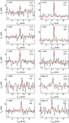 |
Fig. 1 Newlydetected C2O and C3O lines towards: L1544 (panels A, B, C, D, E and F); L1498 (panels G and H); and Elias 18 (panels I and J). Each panel reports the molecule and its transition. Black line: detection; red line: Gaussian fit; dashed vertical line: position of the Gaussian centroid. The detection reported in panel G (performed with the Noto-32 m telescope) was acquired with a lower resolution than that used for the observations reported in the other panels (IRAM-30 m telescope). For clarity we show a larger VLSR scale that allows a better evaluation of the baseline. |
Sources where C2O or C3O was detected.
3 Modelling
The goal of this section is to provide predictions of C2O and C3O abundances, assuming that they are governed by gas-phase chemistry. We describe the astrochemical model that we used (Sect. 3.1), the chemical network (Sect. 3.2), and the resulting predictions obtained varying some crucial parameters (Sect. 3.3).
3.1 Model description
We ran a time-dependent, pure gas-phase chemistry model. To this end, we used the code Nahoon6, modified to improve its usage flexibility. We model a molecular cloud completely shielded from the UV photons of the interstellar radiation field (Av = 100 mag), with a constant density of H nuclei, nH, and a constant temperature T. We started with a partially atomic cloud, meaning that all elements are in the atomic form (neutral or ionized depending on their ionization potential) except hydrogen, which is assumed to be in the molecular form. This mimics the pseudo-evolution of a cloud from neutral to molecular. The chemical composition of the cloud is left to evolve up to 5 × 10⁶ yr.
In Table 2 we report the assumed various initial elemental abundances to study their impact on the C2O and C3O synthesis. We varied either carbon or oxygen abundances to obtain a C/O elemental abundance ratio of 0.4, 0.65, 0.8, and 0.9, respectively. In some cases, the elemental abundances of C and O are different, even if the C/O ratio is maintained equal. We also varied the abundance of elements heavier than carbon. Furthermore, in order to test the sensitivity of the resulting predictions on the crucial parameters of the model, we varied (i) the cloud density between 2 × 104 cm−3 and 1 × 105 cm−3; (ii) the temperature T between 10 and 30 K; and (iii) the cosmic-ray ionization rate ζ between 1 × 10⁻¹⁷ and 1 × 10⁻¹⁶ s−1. Finally, we also ran a few models to simulate the warm regions, called hot corinos, where the icy grain mantles sublimate.
3.2 Chemical network
For the reactions occurring in the gas phase, we used the KIDA 2014 network5, updated to take into account the carbon-chain chemistry described in Loison et al. (2014, 2016), and other reactions involving C-bearing complex species described by Balucani et al. (2015) and Skouteris et al. (2017). Reactions induced by UV photons and by direct collision with cosmic-ray particles are also included. In total, the network contains 507 species connected by 7210 reactions. Figure 2 shows a schematic diagram of the most important reactions involving C2O and C3O. The scheme was obtained a posteriori, looking at the most important formation and destruction reactions within the range of parameters used (see Sect. 3.1). In the figure, all the chemical species that are connected by solid arrows show the formation reactions, while dashed arrows show the destruction pathways. As can be seen, no reaction exists directly connecting C2O and C3O. In other words, the chemical network that we used does not contain any reaction in which C2O is a reactant to form C3O. Also, although a destruction reaction of C3O that produces C2O is included in the network, in practice it is completely negligible, its rate being from 10 to 15 orders of magnitude lower than the other reactions shown in the diagram.
Initial elemental abundances used in the models.
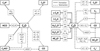 |
Fig. 2 Reaction network including formation (solid lines) and destruction (dashed lines) of C2O and C3O. The boxes intercepting the arrows list the reactants, preceded by a plus symbol, and other products, preceded by a minus symbol, of the relevant reaction in which C2O and C3O are involved. |
3.3 Results of the modelling
As mentioned at the beginning of the section, we ran two classes of models, which approximately described the two classes of objects where C2O and C3O were searched for: cold clouds, and warm gas and hot corinos. The C2O over C3O ratios are shown in Fig. 3 for cold clouds. Simulations obtained for warm gases and hot corinos are shown in Fig. 4.
3.3.1 Cold cloud model
The simulations of gas-phase reactions taking place in a cold cloud allowed us to obtain the C2O/C3O ratios as a function of time (between 102 and 106 yr) for ζ = 1 × 10⁻¹⁶ s−1 and ζ = 1 × 10⁻¹⁷ s−1, and are reported in Fig. 3. The ratios were obtained from the fractional abundances of C2O and C3O calculated by the model. The simulations obtained for ζ = 1 × 10⁻¹⁶ s−1 do not fit the observed C2O/C3O ratios, while for ζ = 1 × 10⁻¹⁷ only in the cases of C/O = 0.65 and 0.9 (blue and magenta curves) are the ratios in agreement with the observed values. However, the agreement is found only in the range ≈103–104 yr, and this is shorter than the timescale of star formation.
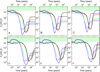 |
Fig. 3 C2O/C3O ratios as a function of time (in years) for ζ = 1 × 10⁻¹⁶ s−1 (top panels, A, B, and C) and for ζ = 1 × 10⁻¹⁷ s−1 (bottom panels, D, E, and F). Panels A and D: 10 K; panels B and E: 20 K; panels C and F: 30 K. The modelwas run for different C/O initial ratios and hydrogen number density. The green boxes represent the lower range of observed ratios (including the errors, see Table 1). Black line: C/O = 0.4, nH = 2 × 104 cm−3; red line: C/O = 0.8, nH = 2 × 104 cm−3; green line: C/O = 0.65, nH = 2 × 104 cm−3; blue line: C/O = 0.65, nH = 2 × 105 cm−3; cyan line: C/O = 0.8, nH = 2 × 105 cm−3; magenta line: C/O = 0.9, nH = 2 × 105 cm−3. |
3.3.2 Warm gas and hot corino models
In Sect. 2, we showed that neither C2O nor C3O is detected in warm sources, shock sites (such as L1157-B1), protocluster objects (OMC-2 FIR4), or hot corinos (IRAS 16293-2422, SVS13A, IRAS 4A). We therefore modelled those regions as well in order to understand why C2O and C3O are absent in warm gas. In fact, it is also important to understand the destruction pathways that can take place under the typical ISM conditions. With this in mind, we used the fractional abundances at the steady state as computed by the modelling at 10 K and for nH = 1 × 107 cm−3 and ζ = 3 × 10⁻¹⁷ s−1 as input abundances. We wanted to know the time required for both molecules to be destroyed at higher temperature and density,to simulate the typical conditions of a protostellar envelope and a hot corino as given by Caselli & Ceccarelli (2012). Also, we modified the reaction network by setting the initial fractional abundance of both C2O and C3O at 10−9. Simulations were performed at 40 K (Fig. 4 panel A) and 100 K (Fig. 4 panel B). The most relevant reactions are reported in Fig. 2. According to the model, even if the initial abundance for both molecules is set to 10−9, at about 102 yr they fall to 10−13 for C3O and to 10−16 for C2O. This trend is noticeable also for simulations at 100 K. For these values of temperature and density, destruction reactions turn out to be more efficient than formation reactions.
4 Experimental results
The experimental results we show in this section are meant to extend the work by Palumbo et al. (2008) and Sicilia et al. (2012) on the effect of ion irradiation on frozen films of carbon monoxide when pure and in mixture with nitrogen under high vacuum and at low temperature. These experiments simulate the effects due to the interaction between low-energy cosmic rays and icy mantles on dust grains, and were performed to study the formation of C2O, C3O, and other carbon-chain oxides in the solid phase after ion irradiation of CO-rich solid mixtures. As recently reviewed by Rothard et al. (2017), fast ions (keV–MeV) impinging on solid samples release their energy through ionizations and excitations of target nuclei along the ion track (i.e. the projectile trajectory). Radicals and molecular fragments are formed which recombine in a very short time (one picosecond or less) giving rise to species not present in the original sample. All these reactions do not occur in thermodynamic equilibrium (e.g. Baratta et al. 2004; Woods et al. 2015).
The experiments presented here were performed in the Laboratory for Experimental Astrophysics (LASp) at INAF-Osservatorio Astrofisico di Catania (Italy). The experimental setup consists in a stainless steel high-vacuum (HV) chamber (P < 10−7 mbar) in which a KBr substrate is placed in thermal contact with a closed-cycle helium cryocooler (CTI) whose temperature can be varied between 16 and 300 K. Pure CO (Aldrich, 99.0%) and CO:N2 (N2 from Alphagaz, 99.9999%) gaseous mixtures were prepared in a mixing chamber and were then admitted in the HV chamber, where they condensed on the substrate at 16 K. After the deposition, the frozen samples were bombarded with 200 keV H+ by means of a 200 kV Danfysik ion implanter connected to the HV chamber. The samples were analysed before, during, and after ion irradiation by a Fourier transform infrared (FTIR) spectrometer (Bruker Vertex 70, 2.5–25 μm, 4000–400 cm−1) to follow the modification induced by the ion beam. For more details on the experimental setup and methods please refer to Palumbo et al. (2008), Sicilia et al. (2012), and Urso et al. (2016).
In Fig. 5 we show the IR spectra acquired during our experiment on ion irradiation of pure solid CO deposited at 16 K. The vibrational band centred at about 2140 cm−1 is due to the fundamentalCO stretching mode (e.g. Urso et al. 2016). Also, the high film thickness allows us to distinguish a broad feature between 2240 and 2160 cm−1 due to a combination of the fundamental CO stretching mode and a lattice vibration. The two blended peaks at about 2092 cm−1 are attributed to the stretching modes of the isotopologues 13C16O and 12C18O, while the 2112 cm−1 band is due to 12C17O (Baratta & Palumbo 1998; Palumbo et al. 2008). The same figure shows the spectrum acquired after irradiation with 200 keV H+ and it is possible to observe the appearance of several new bands. The most intense, observed at 2340 cm−1 (4.27 μm, not shown) is due to the formation of CO2, which is themost abundant species formed after the energetic processing of CO samples (e.g. Trottier & Brooks 2004; Loeffler et al. 2005; Ioppolo et al. 2009; Seperuelo-Duarte et al. 2010). Other bands are due to the ion-induced synthesis of more complex species. The labels in the figure show that most of them have been attributed to several carbon-chain oxides (Jamieson et al. 2006; Palumbo et al. 2008; Sicilia et al. 2012). Among them, the ν1 stretching modes of C2O and C3O lay at 1989 and 2247 cm−1, respectively.We analysed these bands to obtain the column density of both molecules synthesised after ion irradiation of solid CO. We calculated their column densities in units of molecules per square centimetre using Eq. (1),
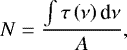 (1)
(1)
where τ(ν) is the optical depth and A is the band strength (cm molecule−1). For both IR modes we used a band strength value of 1 × 10⁻¹⁷ cm molecule−1, as reported by Palumbo et al. (2008). Also, ion irradiation of CO:N2 solid mixtures drives the formation of both C2O and C3O. The IR spectra of different mixtures and the band assignment have already been shown in Sicilia et al. (2012), so we do not report them in this work.
Figure 6 shows the column densities of C2O and C3O with respect to initial CO as a function of ion fluence after irradiation of CO at 16 K. The 2140 cm−1 band being saturated, the CO initial column density was calculated from the sample thickness that was obtained from the interference curve given by a He–Ne laser during the deposition (e.g. Fulvio et al. 2009; Urso et al. 2016), assuming a sample density of 0.8 g cm−3 (Loeffler et al. 2005). The top axis gives an estimation of the time necessary for interstellar ices to undergo the effects observed in laboratory.
In Fig. 7 we show the ratio between the column densities of C2O and C3O as a function of ion fluence per square centimetre that we obtained after ion irradiation of pure CO, CO:N2 = 1:1, CO:N2 = 8:1, and CO:N2 = 1:8 mixtures. It is possible to observe that the higher ratio between C2O and C3O was reachedafter the first ion irradiation step, that is at the lowest fluence value of 3.2 × 10¹² H+ cm−2. We also observed that the C2O/C3O ratio decreases as the fluence increases. The top x-axis gives an estimate of the time (in 106 yr) necessary for interstellar ices to undergo the effects observed in the laboratory. To extrapolate the experimental results to the typical ISM conditions, we followed the method described in Palumbo (2006) and Kaňuchová et al. (2016) and the approximation for cosmic-ion energy reported by Mennella et al. (2003). The timescales on the top x-axis were calculated considering three values of cosmic-ray ionization rate, 1 × 10⁻¹⁵, 1 × 10⁻¹⁶, and 1 × 10⁻¹⁷ s−1, as reported on the right hand side of each axis.
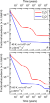 |
Fig. 4 Computations to simulate the destruction of C2O and C3O for a hydrogen number density of 1 × 107 cm−3 and a cosmic-ray ionization rate of 3 × 10⁻¹⁷ s−1 at 40 K (panel A) and 100 K (panel B). Red line: C3O; blue line: C2O. |
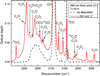 |
Fig. 5 Infrared transmission spectra in optical depth scale of solid CO as deposited at 16 K (black dashed line) and after irradiation with 200 keV H+ (red solid line). All the main vibrational features attributed to carbon-chain oxides are labelled according to Ewing (1989), Maier et al. (1998), Gerakines & Moore (2001), Wang et al. (2002), Jamieson et al. (2006) and Sicilia et al. (2012). (a) Tentative assignment. |
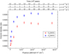 |
Fig. 6 C2O (blue circles)and C3O (red triangles) column densities with respect to the initial CO column density (COi) as a functionof fluence (ions cm−2, bottom x-axis). The top x-axes gives an estimate of the time (in 106 yr) necessary for interstellar ices to undergo the effects observed in the laboratory. Values of cosmic-ray ionization rate used to calculate the timescales are reported near each x-axis in the figure. |
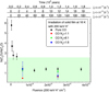 |
Fig. 7 C2O/C3O ratio as a function of fluence (ions cm−2, bottom x-axis) obtained after ion irradiation of pure CO (black squares), CO:N2 = 1:1 mixture (redcircles), CO:N2 = 8:1 (green triangles) and CO:N2 = 1:8 (blue rhombus). Top x-axes give an estimate of the time (in 106 yr) necessary for interstellar ices to undergo the effects observed in the laboratory. Values of cosmic-ray ionization rate used to calculate timescales are reported near each x-axis in the figure. The green box represents the range of observed C2O/C3O ratios in star-forming regions (including the errors. Ratios are given in Table 1. |
5 Discussion
Let us now assemble all the information we obtained from observations, modelling, and laboratory experiments. We have shown that dicarbon and tricarbon monoxide have been detected in TMC-1, L1544, L1498, and Elias 18. The results we obtained modelling the formation and destruction of both molecules predict that their observed abundance ratios cannot be explained only taking into account gas-phase reactions occurring at the typical physical and chemical parameters of star-forming regions. This means that other processes must be involved to explain the presence of C2O and C3O in the gas phase. According to our experimental results, the interaction of cosmic rays with icy mantles is a possible candidate. In fact, we have shown that ion irradiation of CO-rich films produces both C2O and C3O.
Previous studies reported that the C2O and C3O fractional abundance is of the order of 10−11–10−10 (Matthews et al. 1984; Brown et al. 1985; Ohishi et al. 1991; Palumbo et al. 2008; Vastel et al. 2014). In dense molecular clouds, the CO fractional abundance is on the order of 10−4 (e.g. Frerking et al. 1982), thus the carbon-chain oxide abundance with respect to CO is about 10−7–10−6. We carried out a quantitative analysis to infer the amount of both species produced after ion bombardment. Experimental results (see Fig. 6) show that after ion irradiation of solid CO at 16 K the column density of C2O and C3O is 3 × 10⁻³ and 2 × 10⁻³ with respectto the CO initial abundance, respectively. Similarly, Sicilia et al. (2012) found comparable values after ion irradiation of CO:N2 mixtures. Ifwe assume high CO depletion on interstellar ices, and that the C2O/CO and C3O/CO ratios obtained in the experiments are maintained in the gas phase after the icy grain mantles desorption, we find that about 103 yr would be necessary to form the observed column densities for both carbon-chain oxides. Taking into account that the evolution timescale of dense clouds is much longer, the observed gas-phase abundances could be reached even if only a fraction of icy grain mantle desorption occurs or if CO is not completely depleted. Moreover, in Fig. 7 shows that the ratio between C2O and C3O produced after ion irradiation is comparable with the values observed towards the sources under examination. These new results strengthen the hypothesis suggested by Palumbo et al. (2008) that both molecules are produced in the solid phase and then injected into the gas phase because of icy mantle desorption.
Our results are consistent with the fact that both dicarbon and tricarbon monoxide have been detected in cold sources, in which there is no central object warming up the icy mantles. Therefore, we suggest that both molecules are formed in the solid phase and are released to the gas phase after desorption of icy mantles. The sublimation temperature of several Cn O species has been investigated by Jamieson et al. (2006). These authors performed electron irradiation of solid CO at 10 K and a subsequent temperature-programmed desorption (TPD) analysis. They showed that C3O sublimates together with the CO matrix at about 40 K, while CO2, C3O2, and C5O2 sublimate at higher temperature. In addition, desorption could be due to non-thermal processes such as the effects induced by cosmic rays (e.g. Hasegawa & Herbst 1993; Bringa & Johnson 2004; Ivlev et al. 2015).
In more evolved objects, such as IRAS 162593-2422 and L1157-B1, the higher temperature or the presence of shocks cause the complete sublimation of icy grain mantles. As a consequence, the bare grains cannot act as a reservoir of molecules, and we have shown that gas-phase reactions are not able to produce the right amount of C2O and C3O. Therefore, even if both molecules were injected into the gas phase in a previous stage of star formation, after their destruction they cannot be produced in reasonable amounts, as suggested by the modelling we ran at 40 and 100 K shown in Fig. 4. In this discussion, Elias 18 appears to be a possible anomaly. In fact, even if it is a Class I protostar, both molecules have been detected. However, the emission is probably dominated by the cold envelope surrounding the source.
Finally, we would like to report the problems we faced when modelling the gas-phase reactions. As mentioned in Sect. 3 we coupled the Nahoon code with an updated version of the KIDA network in which we included reactions that were recently reported in the literature (Loison et al. 2014; Balucani et al. 2015; Loison et al. 2016; Skouteris et al. 2017). The reaction diagram we proposed in Fig. 2 is based on the results carried out by this model. We have shown 26 reactions that form and destroy both C2O and C3O. But only less than 27% of these reactions have been positively evaluated on the KIDA website, while the remaining are not evaluated and, as reported by Wakelam et al. (2012), are obtained from another database (OSU) that relies more heavily on unstudied radical-neutral reactions. Of course, even if it is a powerful tool to investigate the gas phase of star-forming regions, this lack of both experimental and theoretical data on the possible reactions and their rates could imply huge inaccuracies. Also, neither the standard KIDA network nor our version contains reactions in which C2O is involved as a reactant to produce C3O through a reaction with atomic carbon. A reaction of C2O with C is actually included, but it leads to the destruction of C2O to form C2 and O. Also, a reaction of C2O with C+ determines the charge exchange to give C2O+ and atomic C. Jamieson et al. (2006) proposed a solid phase reaction occurring between C2O and C atoms present in a CO matrix after ion irradiation experiments that gives rise to C3O. Of course, there is no evidence that this reaction could also occur in the gas phase, and its evaluation is not among the purposes of this work.
6 Conclusions
In this work we contribute to the debate on the formation pathways of C2O and C3O in space. The observations reported here were carried out towards several star-forming regions, and for those investigated, both specieswere revealed to exist in the gas phase in colder sources. To interpret the observations we followed a multidisciplinary approach that allowed us to model gas-phase reactions that determine the synthesis of both species and to perform laboratory experiments which simulate the energetic processing of CO-rich icy grain mantles. On the one hand, the model has shown that the low reaction rates to produce both molecules hinder their formation directly in the gas phase. On the other hand, the ion irradiation of CO-rich icy grain mantle analogues has shown that C2O and C3O are efficiently produced in the solid phase and that their ratios agree well with the observed values. Therefore, here we suggest that the synthesis of both species can be attributed to the energetic processing of icy mantles and their subsequent desorption due to non-thermal processes. The model has also shown that once in the gas, both molecules are easily destroyed and their detection would not be possible, unless continuous re-injection from the solid phase occurs. Hopefully, in the near future new observationswill detect both species towards a higher number of sources. This will better constrain the observed C2O/C3O abundance ratio and will allow us to better understand the processes which govern the formation and destruction of carbon chain oxides in space. New experiments and calculations would be necessary to search for the possible link between carbon chain oxides and H- and N-bearing carbon chains that are observed toward various star-forming regions.
Acknowledgements
We are grateful to the referee for the thoughtful reading of the manuscript and for the comments and suggestions which helped us to improve our work. This work has been supported by the Italian Ministero dell’Istruzione, dell’Università e della Ricerca through the grant Progetti Premiali 2012-iALMA (CUP C52I13000140001), by the project PRIN-INAF 2016. The Cradle of Life - GENESIS-SKA (General Conditions in Early Planetary Systems for the rise of life with SKA) and by the COST Action CM1401 Our Astro-chemical History. We also acknowledge the European Union’s Horizon 2020 research and innovation programme from the European Research Council (ERC), for the Project “The Dawn of Organic Chemistry” (DOC), grant agreement No 741002, and from the European MARIE SKODOWSKA-CURIE ACTIONS for the Project “Astro-Chemistry Origins” (ACO), Grant No 811312. This work is based on observations carried out with Noto-32 m telescope operated by INAF-Istituto di Radioastronomia and under project number 194-08 and 014-11 with the IRAM-30 m telescope. IRAM is supported by the INSU/CNRS (France), MPG (Germany) and IGN (Spain). R.G.U. acknowledges the CNES postdoctoral program and the hospitality of the Observatoire de Grenoble during his stay.
Appendix A Sources in which C2O and C3O were searched for
The following tables report the sources in which lines from C2O (Table A.1) and C3O (Table A.2) were searched for together with their rotational transitions and frequencies, spectroscopic parameters, single-dish telescopes used, their beam sizes, and the status of the detection. For the newly detected lines we also report the Tmb, FWHM, Iint and VLSR that are derived from the Gaussian fit. References are reported in the last column. Note that for the ASAI and TIMASSS sources we searched for C2O and C3O in the entireIRAM spectra but here we give only the expected brightest-line frequency.
C2O.
C3O.
References
- Adams, F. C. 2010, ARA&A, 48, 47 [NASA ADS] [CrossRef] [Google Scholar]
- Bachiller, R., Guilloteau, S., Gueth, F., et al. 1998, A&A, 339, L49 [Google Scholar]
- Bachiller, R., Gutiérrez, M., Kumar, M. S. N., & Tafalla, M. 2001, A&A, 372, 899 [NASA ADS] [CrossRef] [EDP Sciences] [Google Scholar]
- Balucani, N., Ceccarelli, C., & Taquet, V. 2015, MNRAS, 449, L16 [Google Scholar]
- Barone, V., Latouche, C., Skouteris, D., et al. 2015, MNRAS, 453, L31 [Google Scholar]
- Baratta, G. A., & Palumbo, M. E. 1998, J. Opt. Soc. Am. A, 15, 12, 3076 [Google Scholar]
- Baratta, G. A., Mennella, V., Brucato, J. R., et al. 2004, J. Raman Spectrosc., 35, 487 [NASA ADS] [CrossRef] [Google Scholar]
- Bottinelli, S., Ceccarelli, C., Lefloch, B., et al. 2004, ApJ, 615, 354 [NASA ADS] [CrossRef] [Google Scholar]
- Bringa, E. M., & Johnson, R. E. 2004, ApJ, 603, 159 [NASA ADS] [CrossRef] [Google Scholar]
- Brown, R. D., Godfrey, P. D., Cragg, D. M., & Rice, E. H. N. 1985, ApJ, 297, 302 [NASA ADS] [CrossRef] [Google Scholar]
- Caselli, P., & Ceccarelli, C. 2012, A&ARv, 20, 56 [NASA ADS] [CrossRef] [MathSciNet] [Google Scholar]
- Caselli, P., Walmsley, C. M., Zucconi, A., et al. 2002, ApJ, 565, 331 [NASA ADS] [CrossRef] [Google Scholar]
- Caselli, P., van der Tak, F. F. S., Ceccarelli, C., & Bacmann, A. 2003, A&A, 403, L37 [NASA ADS] [CrossRef] [EDP Sciences] [Google Scholar]
- Caselli, P., Keto, E., Bergin, E. A., et al. 2012, ApJ, 759, L37 [Google Scholar]
- Ceccarelli, C., Dominik, C., López-Sepulcre, A., et al. 2014, ApJ, 790, L1 [NASA ADS] [CrossRef] [Google Scholar]
- Caux, E., Kahane, C., Castets, A., et al. 2011, A&A, 532, A23 [NASA ADS] [CrossRef] [EDP Sciences] [Google Scholar]
- Charnley, S. B., Kress, M. E., Tielens, A. G. G. M., & Millar, T. J. 1995, ApJ, 448, 232 [NASA ADS] [CrossRef] [Google Scholar]
- Chen, X., Launhardt, R., & Henning, T. 2009, ApJ, 691, 1729 [NASA ADS] [CrossRef] [Google Scholar]
- Chiar, J. E., Adamson, A. J., Kerr, T. H., & Whittet, D. C. B. 1995, ApJ, 455, 234 [NASA ADS] [CrossRef] [Google Scholar]
- Codella, C., Lefloch, B., Ceccarelli, C., et al. 2010, A&A, 518, L112 [NASA ADS] [CrossRef] [EDP Sciences] [Google Scholar]
- Codella, C., Fontani, F., Ceccarelli, C., et al. 2015, MNRAS, 449, L11 [NASA ADS] [CrossRef] [Google Scholar]
- Codella, C., Ceccarelli, C., Bianchi, E., et al. 2016, MNRAS, 462, L75 [NASA ADS] [CrossRef] [Google Scholar]
- Codella, C., Ceccarelli, C., Caselli, P., et al. 2017, A&A, 605, L3 [NASA ADS] [CrossRef] [EDP Sciences] [Google Scholar]
- Comoretto, G., Palagi, F., Cesaroni, R., et al. 1990, A&ASS, 84, 179 [NASA ADS] [Google Scholar]
- Crimer, N., Ceccarelli, C., Lefloch, B., & Faure, A. 2009, A&A, 506, 1229 [NASA ADS] [CrossRef] [EDP Sciences] [Google Scholar]
- Dalgarno, A. 2006, PNAS, 103, 33, 12269 [NASA ADS] [CrossRef] [Google Scholar]
- De Simone, M., Codella, C., Testi, L., et al. 2017, A&A, 599, A121 [NASA ADS] [CrossRef] [EDP Sciences] [Google Scholar]
- Duley, W. W., & Williams, D. A. 1984, Nature, 311, 5987, 685 [NASA ADS] [CrossRef] [Google Scholar]
- Etim, E. E., Gorai, P., Das, A., Chakrabarti, S. K., & Arunan, E. 2016, ApJ, 832, 144 [NASA ADS] [CrossRef] [Google Scholar]
- Ewing, D. W. 1989, J. Am. Chem. Soc., 111, 8809 [CrossRef] [Google Scholar]
- Fontani, F., Codella, C., Ceccarelli, C., et al. 2014, ApJ, 788, L43 [NASA ADS] [CrossRef] [Google Scholar]
- Fontani, F., Ceccarelli, C., Favre, C., et al. 2017, A&A, 605, A57 [NASA ADS] [CrossRef] [EDP Sciences] [Google Scholar]
- Fossé, D., Cernicharo, J., Gerin, M., & Cox, P. 2001, ApJ, 552, 168 [NASA ADS] [CrossRef] [Google Scholar]
- Fraser, H. J., Collings, M. P., Dever, J. W., & McCoustra, M. R. S. 2004, MNRAS, 353, 59 [NASA ADS] [CrossRef] [Google Scholar]
- Frerking, M. A., Langer, W. D., & Wilson, R. W. 1982, ApJ, 262, 590 [NASA ADS] [CrossRef] [Google Scholar]
- Fulvio, D., Sivaraman, B., Baratta, G. A., et al. 2009, Spectrochim. Acta A, 72, 1007 [NASA ADS] [CrossRef] [Google Scholar]
- Garrod, R. T.,& Herbst, E. 2006, A&A, 457, 927 [NASA ADS] [CrossRef] [EDP Sciences] [Google Scholar]
- Gerakines, P. A., & Moore, M. H. 2001, Icarus, 154, 372 [NASA ADS] [CrossRef] [Google Scholar]
- Geyer, C. J. 1992, Stat. Sci., 7, 4, 473 [CrossRef] [Google Scholar]
- Goldsmith, P. F., & Langer, W. D. 1999, ApJ, 517, 209 [NASA ADS] [CrossRef] [Google Scholar]
- Gounelle, M., Shu, F. H., Shang, H., et al. 2006, ApJ, 640, 1163 [NASA ADS] [CrossRef] [Google Scholar]
- Guelin, M., Langer, W. D., & Wilson, R. W. 1982, A&A, 107, 107 [NASA ADS] [Google Scholar]
- Gueth, F., Guilloteau, S., & Bachiller, R. 1998, A&A, 333, 287 [NASA ADS] [Google Scholar]
- Hasegawa, T. I., & Herbst, E. 1993, MNRAS, 261, 83 [NASA ADS] [CrossRef] [Google Scholar]
- Herbst, E., & van Dishoeck, E. F. 2009, ARA&A, 47, 427 [NASA ADS] [CrossRef] [Google Scholar]
- Ioppolo, S., Palumbo, M. E., Baratta, G. A., & Mennella, V. 2009, A&A, 493, 1017 [NASA ADS] [CrossRef] [EDP Sciences] [Google Scholar]
- Irvine, W. M., Goldsmith, P. F., & Hjalmarso, A. 1987, Interstellar Processes, eds. D. Hollenbach & H. Thronson (Dordrecht: Reidel Publishing Company), 561 [Google Scholar]
- Ivlev, A. V., Röcker, T. B., Vasyunin, A., & Caselli, P. 2015, ApJ, 805, 59 [NASA ADS] [CrossRef] [Google Scholar]
- Jaber, A. A., Ceccarelli, C., Kahane, C., et al. 2017, A&A, 597, A40 [NASA ADS] [CrossRef] [EDP Sciences] [Google Scholar]
- Jamieson, C. S., Mebel, A. M., & Kaiser, R. I. 2006, ApJS, 163, 184 [NASA ADS] [CrossRef] [Google Scholar]
- Jøorgensen, J. K., van der Wiel, M. H. D., Coutens, A., et al. 2016, A&A, 595, A117 [NASA ADS] [CrossRef] [EDP Sciences] [Google Scholar]
- Kaifu, N., Ohishi, M., Kawaguchi, K., et al. 2004, PASJ, 56, 69 [NASA ADS] [CrossRef] [Google Scholar]
- Kaňuchová, Z., Urso, R. G., Baratta, G. A., et al. 2016, A&A, 585, A155 [NASA ADS] [CrossRef] [EDP Sciences] [Google Scholar]
- Kuiper, T. B. H., Langer, W. D., & Velusamy, T. 1996, ApJ, 468, 761 [NASA ADS] [CrossRef] [PubMed] [Google Scholar]
- Lefèvre, C., Cabrit, S., Maury, A. J., et al. 2017, A&A, 604, L1 [NASA ADS] [CrossRef] [EDP Sciences] [Google Scholar]
- Lefloch, B., Castets, A., Chernicharo, J., Langer, W. D., & Zylka, R. 1999, A&A, 334, 269 [NASA ADS] [Google Scholar]
- Lefloch, B., Cabrit, S., Busquet, G., et al. 2012, ApJ, 757, L25 [NASA ADS] [CrossRef] [Google Scholar]
- Lefloch, B., Ceccarelli, C., Codella, C., et al. 2017, MNRAS, 469, L73 [NASA ADS] [CrossRef] [Google Scholar]
- Lefloch, B., Bachiller, R., Ceccarelli, C., et al. 2018, MNRAS, 477, 4792 [NASA ADS] [CrossRef] [Google Scholar]
- Loeffler, M. J., Baratta, G. A., Palumbo, M. E., Strazzulla, G., & Baragiola, R. 2005, A&A, 435, 587 [NASA ADS] [CrossRef] [EDP Sciences] [MathSciNet] [Google Scholar]
- Loison, J. C., Wakelam, V., Hickson, K. M., Bergeat, A., & Mereau, R. 2014, MNRAS, 437, 930 [NASA ADS] [CrossRef] [Google Scholar]
- Loison, J. C., Agúndez, M., Marcelino, N., et al. 2016, MNRAS, 456, 4101 [Google Scholar]
- Looney, L. W., Mundy, L. G., & Welch, W. J. 2000, ApJ, 529, 477 [NASA ADS] [CrossRef] [Google Scholar]
- López-Sepulcre, A., Taquet, V., Sánchez-Monge, Á., et al. 2013, A&A, 556, A62 [NASA ADS] [CrossRef] [EDP Sciences] [Google Scholar]
- López-Sepulcre, A., Jaber, A. A., Mendoza, E., et al. 2015, MNRAS, 449, 2438 [NASA ADS] [CrossRef] [Google Scholar]
- López-Sepulcre, A., Sakai, N., Neri, R., et al. 2017, A&A, 606, A121 [NASA ADS] [CrossRef] [EDP Sciences] [Google Scholar]
- Maier, G., Riesenauer, H. P., Schafer, U., & Balli, H. 1988, Angew. Chem., 100, 590 [CrossRef] [Google Scholar]
- Mangum, J. G., & Wootten, A. 1990, A&A, 239, 319 [NASA ADS] [Google Scholar]
- Matthews, H. E., Irvine, W. M., Friberg, P., Brown, R. D., & Godfrey, P. D. 1984, Nature, 310, 125 [NASA ADS] [CrossRef] [Google Scholar]
- McGuire, B., Carroll, P. B, Loomis, R. A., et al. 2013, ApJ, 774, 56 [NASA ADS] [CrossRef] [Google Scholar]
- Mennella, V., Baratta, G. A., Esposito, A., et al. 2003, ApJ, 587, 727 [NASA ADS] [CrossRef] [EDP Sciences] [Google Scholar]
- Miller, J. S. 1970, ApJ, 191, L95 [NASA ADS] [CrossRef] [Google Scholar]
- Mundy, L. G., Wootten, A., Wilking, B. A., Blake, G. A., & Sargent, A. I. 1992, ApJ, 385, 306 [NASA ADS] [CrossRef] [Google Scholar]
- Müller, H. S. P., Thorwirth, S., Roth, D. A., et al. 2001, A&A, 370, L49 [NASA ADS] [CrossRef] [EDP Sciences] [Google Scholar]
- Müller, H. S. P., Schlöder, F., Stutzki, J., et al. 2005, J. Mol. Structure, 742, 215 [CrossRef] [Google Scholar]
- Nummelin, A., Whittet, D. C. B., Gibb, E. L., Gerakines, P. A., & Chiar, J. E. 2001, ApJ, 558, 185 [NASA ADS] [CrossRef] [Google Scholar]
- Ohishi, M., Ishikawa, S., Yamada, C., et al. 1991, ApJ, 380, L39 [NASA ADS] [CrossRef] [Google Scholar]
- Palumbo, M. E. 2006 A&A, 453, 903 [NASA ADS] [CrossRef] [EDP Sciences] [MathSciNet] [Google Scholar]
- Palumbo, M. E., & Strazzulla, G. 1993, A&A, 269, 568 [NASA ADS] [Google Scholar]
- Palumbo, M. E., Leto, P., Siringo, C., & Trigilio, C. 2008, ApJ, 685, 1033 [NASA ADS] [CrossRef] [Google Scholar]
- Pickett, H. M., Poynter, R. L., Cohen, E. A., et al. 1998, J. Quant. Spectr. Rad. Transf., 60, 883 [NASA ADS] [CrossRef] [Google Scholar]
- Podio, L., Codella, C., & Gueth, F. 2016, A&A, 593, L4 [NASA ADS] [CrossRef] [EDP Sciences] [Google Scholar]
- Quénard, D., Vastel, C., Ceccarelli, C., et al. 2017, MNRAS, 470, 3194 [NASA ADS] [CrossRef] [Google Scholar]
- Rothard, H., Domaracka, A., Boduch, P., et al. 2017, J. Phys. B. At. Mol. Opt. Phys., 50, 062001 [Google Scholar]
- Santangelo, G., Codella, C., Cabrit, S., et al. 2015, A&A, 584, A126 [NASA ADS] [CrossRef] [EDP Sciences] [Google Scholar]
- Seperuelo Duarte, E., Domaracka, A., Boduch, P., et al. 2010, A&A, 512, A71 [NASA ADS] [CrossRef] [EDP Sciences] [Google Scholar]
- Shimajiri, Y., Takahashi, S., Takakuwa, S., Saito, M., & Kawabe, R. 2008, ApJ, 683, 255 [NASA ADS] [CrossRef] [Google Scholar]
- Shimajiri, Y., Sakai, T., Kitamura, Y., Tsukagoshi, T., Saito, M., et al. 2015, ApJS, 221, 31 [CrossRef] [Google Scholar]
- Sicilia, D., Ioppolo, S., Vindigni, T., Baratta, G. A., & Palumbo, M. E. 2012, A&A, 543, A155 [NASA ADS] [CrossRef] [EDP Sciences] [Google Scholar]
- Sims, I. R., & Smith, W. M. 1995, Annu. Rev. Phys. Chem., 46, 109 [NASA ADS] [CrossRef] [Google Scholar]
- Skouteris, D., Vazart, F., Ceccarelli, C., et al. 2017, MNRAS, 468, L1 [NASA ADS] [Google Scholar]
- Strazzulla, G., Brucato, J. R., Palumbo, M. E., & Satorre, M. A. 1997, A&A, 321, 618 [NASA ADS] [Google Scholar]
- Tegler, S. C., Weinteraud, D. A., Rettig, T. W., et al. 1995, ApJ, 439, 279 [NASA ADS] [CrossRef] [Google Scholar]
- Tenenbaum, E. D., Aponi, A. J., Ziurys, L. M., et al. 2006, ApJ, 649, L17 [NASA ADS] [CrossRef] [Google Scholar]
- Tielens, A. G. G. M., & Hagen, W. 1982, A&A, 114, 245 [Google Scholar]
- Tielens, A. G. G. M., Tokunaga, A. T., Geballe, T. R., & Baas, F. 1991, ApJ, 381, 181 [NASA ADS] [CrossRef] [PubMed] [Google Scholar]
- Tobin, J. J., Looney, L. W., Li, Z.-Y., et al. 2016, ApJ, 818, 73 [NASA ADS] [CrossRef] [Google Scholar]
- Trottier, A., & Brooks, R. L. 2004, ApJ, 612, 1214 [NASA ADS] [CrossRef] [Google Scholar]
- Turner, B. E., Herbst, E., & Terzieva, R. 2000, ApJS, 126, 427 [NASA ADS] [CrossRef] [Google Scholar]
- Urso, R. G., Scirè, C., Baratta, G. A., Compagnini, G., & Palumbo, M. E. 2016, A&A, 594, A80 [NASA ADS] [CrossRef] [EDP Sciences] [Google Scholar]
- van Ravenzwaaij, D., Cassey, P., & Brown, S. D. 2018, Psychon. Bull. Rev., 25, 143 [Google Scholar]
- Vastel, C., Ceccarelli, C., Lefloch, B., & Bachiller, R. 2014, ApJ, 795, L2 [Google Scholar]
- Vastel, C., Bottinelli, S., Caux, E., Glorian, J.-M., & Boiziot, M. 2015, Proceedings of the Annual meeting of the French Society of Astronomy and Astrophysics, eds. F. Martins, S. Boissier, V. Buat, L. Cambrésy, & P. Petit, 313 [Google Scholar]
- Vastel, C., Kawaguchi, K., Quénard, D., et al. 2018a, MNRAS, 474, L76 [NASA ADS] [CrossRef] [Google Scholar]
- Vastel, C., Quénard, D., Le Gal, R., et al. 2018b, MNRAS, 478, 5514 [NASA ADS] [CrossRef] [Google Scholar]
- Vazart, F., Latouche, C., Skouteris, D., Balucani, N., & Barone, V. 2015, ApJ, 810, 111 [Google Scholar]
- Wakelam, V., Herbst, E., Loison, J. C., et al. 2012, ApJS, 199, 21 [NASA ADS] [CrossRef] [Google Scholar]
- Wang, H. Y., Lu, X., Huang, R. B., & Zheng, L. S. 2002, J. Mol. Struct., 593, 187 [CrossRef] [Google Scholar]
- Webber, W. E. 1998, ApJ, 506, 329 [NASA ADS] [CrossRef] [Google Scholar]
- Willacy, L., Langer, W. D., & Velusamy, T. 1998, ApJ, 507, L171 [NASA ADS] [CrossRef] [Google Scholar]
- Woods, P. M., Occhiogrosso, A., Viti, S., et al. 2015, MNRAS, 450, 1256 [NASA ADS] [CrossRef] [Google Scholar]
- Woon, D. E., & Herbst, E. 2009, ApJS, 185, 273 [NASA ADS] [CrossRef] [Google Scholar]
- Wootten, A. 1989, ApJ, 337, 858 [NASA ADS] [CrossRef] [Google Scholar]
- Wootten, A., Bozyan, E. P., Garrett, D. B., Loren, R. B., & Snell, R. 1980, ApJ, 239, 844 [NASA ADS] [CrossRef] [Google Scholar]
- Yamamoto, S., Saito, S., Ohishi, M., et al. 1987, ApJ, 322, L55 [NASA ADS] [CrossRef] [Google Scholar]
The source selection adopted and a detailed description of the targets is reported in Sect. 2.1.
We excluded IRC +10216 from the discussion as it is an asymptotic giant branch (AGB) carbon-rich star (e.g. Miller 1970).
The original code is publicly available at http://kida.obs.u-bordeaux1.fr (Wakelam et al. 2012).
All Tables
All Figures
|
Fig. 1 Newlydetected C2O and C3O lines towards: L1544 (panels A, B, C, D, E and F); L1498 (panels G and H); and Elias 18 (panels I and J). Each panel reports the molecule and its transition. Black line: detection; red line: Gaussian fit; dashed vertical line: position of the Gaussian centroid. The detection reported in panel G (performed with the Noto-32 m telescope) was acquired with a lower resolution than that used for the observations reported in the other panels (IRAM-30 m telescope). For clarity we show a larger VLSR scale that allows a better evaluation of the baseline. |
| In the text | |
|
Fig. 2 Reaction network including formation (solid lines) and destruction (dashed lines) of C2O and C3O. The boxes intercepting the arrows list the reactants, preceded by a plus symbol, and other products, preceded by a minus symbol, of the relevant reaction in which C2O and C3O are involved. |
| In the text | |
|
Fig. 3 C2O/C3O ratios as a function of time (in years) for ζ = 1 × 10⁻¹⁶ s−1 (top panels, A, B, and C) and for ζ = 1 × 10⁻¹⁷ s−1 (bottom panels, D, E, and F). Panels A and D: 10 K; panels B and E: 20 K; panels C and F: 30 K. The modelwas run for different C/O initial ratios and hydrogen number density. The green boxes represent the lower range of observed ratios (including the errors, see Table 1). Black line: C/O = 0.4, nH = 2 × 104 cm−3; red line: C/O = 0.8, nH = 2 × 104 cm−3; green line: C/O = 0.65, nH = 2 × 104 cm−3; blue line: C/O = 0.65, nH = 2 × 105 cm−3; cyan line: C/O = 0.8, nH = 2 × 105 cm−3; magenta line: C/O = 0.9, nH = 2 × 105 cm−3. |
| In the text | |
|
Fig. 4 Computations to simulate the destruction of C2O and C3O for a hydrogen number density of 1 × 107 cm−3 and a cosmic-ray ionization rate of 3 × 10⁻¹⁷ s−1 at 40 K (panel A) and 100 K (panel B). Red line: C3O; blue line: C2O. |
| In the text | |
|
Fig. 5 Infrared transmission spectra in optical depth scale of solid CO as deposited at 16 K (black dashed line) and after irradiation with 200 keV H+ (red solid line). All the main vibrational features attributed to carbon-chain oxides are labelled according to Ewing (1989), Maier et al. (1998), Gerakines & Moore (2001), Wang et al. (2002), Jamieson et al. (2006) and Sicilia et al. (2012). (a) Tentative assignment. |
| In the text | |
|
Fig. 6 C2O (blue circles)and C3O (red triangles) column densities with respect to the initial CO column density (COi) as a functionof fluence (ions cm−2, bottom x-axis). The top x-axes gives an estimate of the time (in 106 yr) necessary for interstellar ices to undergo the effects observed in the laboratory. Values of cosmic-ray ionization rate used to calculate the timescales are reported near each x-axis in the figure. |
| In the text | |
|
Fig. 7 C2O/C3O ratio as a function of fluence (ions cm−2, bottom x-axis) obtained after ion irradiation of pure CO (black squares), CO:N2 = 1:1 mixture (redcircles), CO:N2 = 8:1 (green triangles) and CO:N2 = 1:8 (blue rhombus). Top x-axes give an estimate of the time (in 106 yr) necessary for interstellar ices to undergo the effects observed in the laboratory. Values of cosmic-ray ionization rate used to calculate timescales are reported near each x-axis in the figure. The green box represents the range of observed C2O/C3O ratios in star-forming regions (including the errors. Ratios are given in Table 1. |
| In the text | |
Current usage metrics show cumulative count of Article Views (full-text article views including HTML views, PDF and ePub downloads, according to the available data) and Abstracts Views on Vision4Press platform.
Data correspond to usage on the plateform after 2015. The current usage metrics is available 48-96 hours after online publication and is updated daily on week days.
Initial download of the metrics may take a while.