| Issue |
A&A
Volume 693, January 2025
|
|
|---|---|---|
| Article Number | A236 | |
| Number of page(s) | 8 | |
| Section | Astrophysical processes | |
| DOI | https://doi.org/10.1051/0004-6361/202451754 | |
| Published online | 05 February 2025 | |
Simulation of weak electron beam injection into plasma with open boundary conditions
Institute of Solar-Terrestrial Physics SB RAS, 664033 Irkutsk, Russia
⋆ Corresponding author; annenkov.phys@gmail.com
Received:
1
August
2024
Accepted:
19
December
2024
Context. Different high-energy events lead to the generation of electron beams in the solar atmosphere as well as in planetary magnetospheres. The propagation of these beams through space plasma becomes a main source of non-thermal emission, primarily on the harmonics of the fundamental plasma frequency. Due to the high level of non-linearity and the complexity of such systems, theoretical studies of them are largely based on numerical simulations. However, it is still common practice to use a simplified model in which periodic boundary conditions for fields and particles are used to simulate an infinite plasma.
Aims. In this work, the first attempt at high-resolution studies of the dynamics of a weak beam in space plasma using a model with open boundary conditions is reported. The general results of the simulations are compared with those obtained previously using the approximation of infinite plasma.
Methods. The continuous injection of an electron beam with an average velocity of vb = 0.25c (c – speed of light) and a relative density of nb/n0 = 5 ⋅ 10−4 (n0 – plasma density) into an unmagnetised plasma was simulated in a quasi-1D approximation using a collisionless electromagnetic particle-in-cell code. The background plasma was initially homogeneous and consisted of electrons and protons with the real mass ratio. The total simulation time was 10 000 ωp0−1, where ωp0 is the Langmuir frequency for the given n0.
Results. The present simulations demonstrate the formation of a spatially localised Langmuir turbulence in the close vicinity of the beam injection site. The continuous injection of fresh beam particles increases the amplitude of the plasma waves to values larger than those possible when simulating the same parameters in a simplified model. Plasma waves in this region turn out to be unstable against the modulation instability, so the formation of density wells followed by plasma wave trapping is observed. Some of the beam particles are significantly accelerated by previously arisen plasma waves. On average, only 10% of the beam energy gets lost in the system, but the distribution function is transformed into a flat-top form with a supra-thermal tail.
Conclusions. The obtained results demonstrate several significant differences from the results of simulations using the approximation of infinite plasma. This fact emphasises the importance of using of a more realistic model for simulations of beam-plasma systems. In addition, using the model with open boundaries, in contrast to the simplified model, will allow us to correctly investigate the influence of not only random gradients of the plasma parameters, but also regular ones.
Key words: acceleration of particles / plasmas / methods: numerical / Sun: flares / Sun: radio radiation / solar wind
© The Authors 2025
 Open Access article, published by EDP Sciences, under the terms of the Creative Commons Attribution License (https://creativecommons.org/licenses/by/4.0), which permits unrestricted use, distribution, and reproduction in any medium, provided the original work is properly cited.
This article is published in open access under the Subscribe to Open model. Subscribe to A&A to support open access publication.
1. Introduction
The interaction of electron beams with plasmas is one of the fundamental processes of plasma physics. Electron beams have a wide range of applications in laboratory plasma systems; for example, for plasma heating (Burdakov et al. 2007), emission generation (Arzhannikov et al. 2020), ionisation of neutral gas, and acceleration of electrons (Soldatkina et al. 2022). Recent experiments (Schönlein et al. 2016) on irradiation of metal wires demonstrate the possibility of creating electron beams inside such targets and heating them to temperature of dozens of electron volts. Such experiments should allow one to get insights into warm density matter evolution, which is relevant not only for research in the area of inertial fusion, but also for studies of dense stars. Being accelerated during various high-energy events in the solar atmosphere (Aschwanden 2002; Klein et al. 2005; Jebaraj et al. 2023; Khotyaintsev et al. 2019), electron fluxes cause a wide variety of electromagnetic (EM) emission processes (Ginzburg & Zheleznyakov 1958; Melrose 1980; Robinson & Cairns 2000; Reid & Ratcliffe 2014) and also possibly have an impact on artificial satellites (Hapgood 2016).
Great progress in the theoretical description of the beam-plasma interactions has been made in over a century of plasma research. However, an analytical description of these processes is strictly limited to different simplified cases, while many practically important regimes can be investigated only through numerical simulations, mainly using the particle-in-cell (PIC) approach (Dawson 1983). With rapid growth in computing power, it has become possible to simulate vast plasma systems using different numerical schemes with high resolution on large timescales. However, for real systems to be adequately described by means of simulations, it is also necessary to choose the correct model of simulation box. By now, the majority of PIC simulations of solar beam-plasma systems (e.g. Thurgood & Tsiklauri 2016; Henri et al. 2019; Zhang et al. 2022; Krafft & Savoini 2023; Li et al. 2024) are still performed in simplified geometry with periodic boundary conditions, which correspond to the infinite plasma case.
The model of infinite plasma is actually assumed in the majority of analytical estimates of different plasma processes; for example, in the classic theory of beam-plasma instability (Akhiezer & Fainberg 1949; Bohm & Gross 1949). That makes using a similar model in numerical simulations the best choice for the verification of many theoretical concepts. The model of infinite plasma can be realised for any spatial geometry via implementation of the periodic boundary conditions for fields and particles. Figure 1 demonstrates the scheme of the simulation box in 2D geometry for infinite plasma. Due to the periodic boundary conditions, the particles actually move on the surface of a torus, while the spectrum of EM fields become restricted by the spatial size of the simulation box. Typical initial conditions for beam-plasma systems in this model are as follows. Particles of the plasma species (ions and electrons) are distributed uniformly over the simulation box. In the same manner, electrons of the beam are placed in all space with the initial temperature distribution and directed velocity. Meanwhile, electrons of plasma have not only a temperature spread, but also some mean velocity in the opposite direction to the beam in order to construct a compensating current. After such an initiation, we can observe the evolution of the system in time. The beam drives various instabilities (Bret et al. 2008). Simulations usually correctly reproduce predictions of the theories on the linear stage. Then, one can observe the vast majority of non-linear processes. However, such initial conditions do not actually correspond to real beam-plasma systems. Whether in experimental or natural conditions, we always have a definite source for the beam particles, which propagate through plasma. For example, solar radio bursts can be generated by particle fluxes, which originate far from the radio emission source. On the one hand, this means that these beams will have a complicated distribution function due to their interaction with plasma before the emission site. On the other hand, the emission site is a plasma region of finite size with an inflow of beam particles from one side and an outflow from the other. These particles interact with the plasma, build up different waves, and leave the area of interest. The duration of typical radio bursts is much longer than the plasma period in the corresponding area. So, from the point of view of now-available beam-plasma simulations with a length of up to 10 000 inverse plasma frequencies  , such a system will look like the constant injection of an electron beam in a finite size plasma column with open boundaries in the direction of beam propagation (Fig. 2). In this model, we correctly reproduce the real situation of a constant inflow of new particles into the system, while in the model of infinite plasma the electron beam has only a limited amount of initial energy and throughout the entire non-linear stage realistic energy income is absent. Another major difference between these models is the possibility that EM waves leave the system in the case of open boundary conditions, while in infinite plasma these waves remain in the simulation box and continue to interact with particles and other waves.
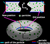 |
Fig. 1. Schematic representation of a simulation box for infinite plasma. The cyan arrow indicates the path of one particle, which passes through all periodic boundaries. |
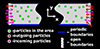 |
Fig. 2. Simulation box with open boundaries in the longitudinal direction (x axis) and periodic boundaries in the transverse one (y axis). Beam particles are injected into the system through the left edge. They cause a return current of plasma electrons and leave the system through the right border. The flux of all of the plasma particles is maintained in a self-consistent manner on both sides. |
The necessity to use a simulation box with open boundary conditions and a continuously injected beam in proper simulations of processes in space plasma was clear dozens of years ago (Büchner et al. 2003), but for a long time such simulations were limited to different simplified cases. For example, in work by Mandrake et al. (2000) a 2.5D electrostatic code was used, and a 1D spatial geometry for dense beams was used by Lizunov et al. (2002). The simulation of low dense electron beams was hampered by the much larger amount of computational resources required for the model with beam injection. In this case, we have to use a simulation box long enough to fit the full relaxation length, LR ∝ vb/Γ, where vb is the mean beam velocity, and Γ the growth rate of the most unstable plasma mode. The lower the Γ, the longer the system we have to use, and therefore the more computational resources are needed. This is the case for the low-density beam or the hot temperature of the electrons in the system. On the other hand, when we use the periodic boundary conditions to simulate beam-plasma interactions, a simulation box of even one plasma wavelength is enough to observe beam-plasma instability and the formation of plasma waves. A further increase in the length of the simulation box in the direction of beam propagation will only increase the spectrum of waves for which existence is possible in the system. This is of course important if we are interested in investigating non-linear wave transformations in long-term dynamics.
In recent years, we have observed a rapid growth in available computation power, which is opening up huge possibilities for simulating plasma processes. In particular, at the Budker Institute of Nuclear Physics, we were able to switch to PIC simulations using the model with open boundaries and continuously injected beams after developing a code for then-new general-purpose graphical processing units (GPGPUs) (Lindholm et al. 2008), which turned out to be a perfect solution for highly parallelised tasks like plasma simulations. Over the next decade, we investigated a lot of beam plasma systems in 2D spatial geometry, mainly in the context of plasma emission tasks (Annenkov et al. 2016a, 2018, 2019; Annenkov et al. 2020, 2024), electron acceleration in an open magnetic trap (Timofeev et al. 2022), and examinations of the influence of plasma density gradients (Annenkov & Volchok 2023). The possibility of simulating large-scale gradients is one more fundamental advantage of the open-boundary model over the infinite one. Other recent examples of successful usage of the model with open boundaries include the work by Nishikawa et al. (2023), in which relativistic jet injection into a plasma was simulated using the TRISTAN code (Spitkovsky 2005) on times up to 900  in full 3D spatial geometry, and the work by Kumar et al. (2022) in which EM emission of colliding electron beams was simulated by the EPOCH code (Arber et al. 2015) in 2D geometry. However, all of the studies mentioned above deal with relatively dense and mostly high-energy electron beams.
This work pursues several objectives. The first one is to investigate the relaxation process of a weak electron beam in a solar wind plasma using PIC simulations in a realistic model with open boundary conditions. For this, the numerical model and approaches being approbated in the context of laboratory experiments were used. The second objective is to demonstrate and discuss main differences of the obtained results with the simulations using infinite model. For this, the system parameters were chosen according to the parameters actively used for PIC simulations of electron beams in solar wind plasmas in the infinite plasma approximation by Krafft & Savoini (2021, 2022, 2023, 2024). The final objective is to briefly discuss other possible approaches to numerical simulations of beam-plasma systems in the context of solar-related problems.
2. Numerical model and parameters
To simulate a beam-plasma system, the 2D3V Cartesian PIC code with a standard numerical scheme was used. It is based on the Yee (1966) solver of Maxwell equations for EM fields, the Boris (1970) scheme for solving the equation of motion for collisionless macro-particles with a parabolic form factor, and the charge-conserving Esirkepov (2001) scheme for calculations of currents.
The proper open boundary conditions should support several features: they have to first be able to remove from the simulation box outgoing particles and EM waves; second, imitate the presence of real particles and fields beyond the edge of the simulation plasma slab; and third, realise the correct inflow of particles into the simulation area. The former feature is crucial not only for sustaining the thermal flow of plasma particles, but also to maintain the correct return current, which should compensate for the current of the beam. Moreover, this compensation should be realised in a self-consistent manner, because beam distribution and mean velocity can be changed dramatically and unpredictably during propagation in plasma. In the code in use, the self-consistent plasma buffers are realised. They fit these requirements and are described in Annenkov et al. (2018).
The simulations were performed using four Nvidia A100 GPGPU. The scheme of the simulation box is presented in Fig. 2. Open boundary conditions were imposed in the longitudinal direction (x axis).
The injected electron beam has a relative density of nb/n0 = 5 ⋅ 10−4, where n0 is the density of the unperturbed plasma. This beam density is an order or two higher than the typical values measured in the solar wind. However, when such a density is used in simulations with periodic boundaries the resulting level of Langmuir turbulence becomes comparable to in situ measurements. This is caused by the limited amount of energy in the simulated beam and absence of fresh particles coming into the system, as is the case in real beam-plasma systems. The long-term non-linear dynamic of plasma waves in an infinite plasma system should also differ, because plasma waves do not have the possibility to interact with fresh beam particles and their associated oscillation modes. The mean velocity of the beam is vb = 0.25c (≈17 keV), where c is the speed of light. All particles in the system initially have a Maxwell distribution:
![$$ \begin{aligned} f(p)\exp \left[-\dfrac{\left(p-p_0\right)^2}{\Delta p^2}\right],\end{aligned} $$](/articles/aa/full_html/2025/01/aa51754-24/aa51754-24-eq4.gif)
where p is the momentum of the particles in units of mec, me is the rest mass of an electron (511 keV), p0 is the mean momentum, and  , where
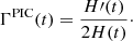
  . For electrons in the plasma and the beam, the initial temperature is Te = 320 eV, which corresponds to a thermal velocity of vT ≈ 0.1vb. For ions in the plasma, the temperature Ti = 0.1Te was used. Such a ratio for the temperatures of plasma components will prevent damping of ion acoustic waves. In contrast to the infinite plasma model, it is not necessary to artificially compensate for the beam current by giving the plasma electrons an average velocity in the direction opposite to the beam direction. The external magnetic field was set to zero. The calculation of the full unstable spectrum in this beam-plasma system using the DispLib code (Annenkov et al. 2021) demonstrates (Fig. 3) the domination of purely longitudinal modes. The maximum growth rate, Γ/ωp0 ≈ 1.4 ⋅ 10−2, corresponds to the wave number, k∥ = 4.29 ωp0/c, where ∥ indicates a direction along the beam axis.
 |
Fig. 3. a) Growth rate map for the beam-plasma instability, Γ(k∥, k⊥). The green line, k⊥ = k⊥(k∥), marks the local maximal growth rate. b) Growth rate for longitudinal modes, Γ(k∥, 0). c) Growth rate on the line of the maximum, Γ(k⊥). |
The relaxation length of electron beams with low relative density imposes a requirement to use a relatively long simulation box. Moreover, it is also imposes a restriction on the minimal simulation time. It has to be long enough to fit the whole linear stage of the beam-plasma instability and give the ability to study the non-linear stage. Fulfilling both these conditions requires additional computation power. Since the most unstable beam-plasma modes are purely longitudinal, it is possible to restrict first studies to 1D regime. So, in this work, the simulations are limited to the quasi-1D case. The simulation box has Ny = 4 cells and periodic boundary conditions in the transverse direction. Such a choice allows us to study the main features of the beam-plasma instability with high resolution in space and time on large spatial scales and timescales, but prohibits the investigation of non-linear process, which involve transverse modes. Due to these restrictions, the present simulations do not allow for deep studies of the EM emission generation, but make possible an investigation of the evolution of the distribution functions of a plasma and a beam, as well as the growth and evolution of longitudinal plasma oscillations.
The longitudinal size of the simulation box is Nx = 3600 cells, which corresponds to a length of Lx = 72 c/ωp0 = 2880 λD, where λD = vT/ωp0 is the Debye length. It should be noted that for simulations with open boundary conditions one should choose the size of the area with an extra space, because processes near the injector (e.g. the formation of strong density gradients Annenkov et al. 2019) can shift the area of intensive beam-plasma interactions further from the injector. For each particle species, Np = 2025 macro-particles per cell were used. The size of cells is Δx = Δy = 0.02 c/ωp0 and the time step is Δt = 0.01  . The total simulation time is 10 000
  . Such small spatial and time steps enable all plasma oscillations to be investigated with high precision, while the long simulation time makes it possible to catch the process caused by the ion dynamic. At the initial time step, all particles of the plasma electrons and ions with the same densities, ne = ni = n0, are distributed across the simulation box with the initial thermal spread.
Later in the text, all quantities are presented in a dimensionless form. Plasma and beam particle densities were calculated in units of n0; all frequencies in 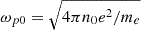 ; wave numbers in ωp0/c; lengths in c/ωp0; time in
  ; EM fields measured in units of mecωp0/c; and particle velocities in the speed of light, c. Since the conversion was based on the initial density of plasma, n0, all of the simulation results can be applied to different real systems with various plasma densities. For example, for coronal plasma with n0 = 1010 cm−3, the unit of length is 1 c/ωp0 ≈ 5.3 cm and the unit of time is
  ns, while for solar wind plasma with n0 = 105 cm−3, the unit of length is 1 c/ωp0 ≈ 17 m and the unit of time is
  ns. For convenience, the conversion factors from dimensionless to dimensional units for various densities are available in Fig. A.1 in the appendix. However, the results of the current simulation are applicable only to systems with temperatures similar to ones we have chosen.
3. Simulation results
First, we shall discuss the process qualitatively. In Fig. 4, snapshots of the simulation results are presented. At the initial stage (Fig. 4 top), the electron beam undergoes two-stream instability and builds up plasma waves with the phase velocity of the beam particles. The spatially localised region with high frequency field oscillations is formed in the vicinity of the beam injection site (Fig. 5). The presence of continuously injected fresh beam electrons leads to the rise in the wave amplitude. It turns out that this amplitude along with the other system parameters is enough to make plasma waves unstable against the modulation instability (Vedenov & Rudakov 1964; Zakharov 1972; Thornhill & ter Haar 1978). Later time moments demonstrate the formation of ion density wells and the capturing of the plasma waves inside them. Such trapped oscillations fall out from the resonance with the electron beam and gradually expend their energy on well deepening. After they have burned out, regions with high density gradients are formed. Such gradients, in turn, prevent the development of beam-plasma instabilities. After some time, these density perturbations can be smoothed out by thermal ion dynamics, and conditions for instability development return. This process is described in more detail in the work Annenkov et al. (2019), in which it is also demonstrated that the formation of such a longitudinal modulation provides the necessary conditions for the beam-plasma antenna mechanism (Annenkov et al. 2016b; Timofeev et al. 2016) and the generation of EM emission near the plasma frequency and its second harmonic. Moreover, as can be seen from phase portraits in Fig. 4, the observed waves provide appropriate conditions for acceleration of the beam electrons to supra-thermal velocities.
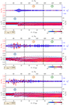 |
Fig. 4. Simulation results at several moments in time. Top: Density of the ions (red line), different phases of one plasma oscillation (blue lines). Bottom: Phase space, f(vx, x), of the beam. The corresponding video is available online. |
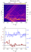 |
Fig. 5. Top: Evolution of the field, Ex, maximum in space and time. Bottom: Time dependence of the field, Ex, maximum (blue) and its position (brown). The horizontal blue line marks the average value of the longitudinal electric field, Ex, in the plasma wave during the non-linear stage. |
Now we shall look at the results in more detail. In Fig. 6, the growth rate of the beam instability in simulations is shown. It was calculated using the energy, H(t), of the electric field in the whole area as follows:
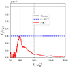 |
Fig. 6. Dependence of the instability growth rate, Γ, on time. The horizontal solid black line indicates a prediction of the linear theory. |
This graph allows us to define the boundary between two stages of the system evolution. At time moment t0 = 900  , the growth rate dependence shift from rapid changes to a flat-like regime. Before t0, the regime of beam-plasma instability is almost linear and after it is non-linear. As we shall see further, this boundary also appears on the time dependencies of other integral system parameters. One more important difference between simulations in the infinite plasma model and the one with open boundaries should also be noted. In the first model, we initially placed in the simulation box all beam particles with the initial distribution function. Therefore, all beam electrons participate in the instability development at once, in good agreement with the predictions of the linear theory (Fig. 3). In the second model, the realistic situation when the fastest particles from the initial velocity distribution function (VDF) reach new plasma layers takes place. In this situation, the head of the beam build up plasma waves not in agreement with the predictions of linear theory for the whole initial distribution and the core of the beam enters in plasma layers with already existent plasma waves. This makes even the linear stage of the beam-plasma instability more complicated.
In Fig. 7, the distribution function, f(vx), of all electrons (plasma and beam) at different time moments and in various areas of the simulation box are presented. Plasma electrons are heated, but their distribution remains Maxwellian. At the end of the linear stage (t ⋅ ωp0 = 900), all distributions have areas with a positive slope of ∂f/∂vx, and therefore continue to be unstable. At later moments, this is only the case for the first area, which is located near the beam injector site. However, at later moments, we can see significant acceleration of some beam particles to velocities far above the thermal speed. At the beginning, 20% of the beam energy is contained in supra-thermal particles (Fig. 8). During the simulation, that percentage increases to 50%. The average value over the entire non-linear stage in regions 1 and 2 turns out to be near 35%. This result exceeds by 5% the same value from the simulation in the infinite model, even for the initially inhomogeneous plasma density. It is also worth noting that in the model with open boundaries we obtained such an acceleration during the short time in which the beam particle was present in the system before leaving it, while in the model with periodic boundaries each particle remains in the system for the entire simulation time and has many chances to be accelerated. Another parameter that can be compared with the simulations by Krafft & Savoini (2023) is the fraction of beam energy that was transferred to waves. In the case of infinite plasma with an inhomogeneous initial density, it turns out to be ≈10%. The same value appears to be in the present simulations (Fig. 9). However, 10% is only the average value. We also can see the number of time moments when beam particles leaving the system significantly increase their energy in comparison with the time of injection.
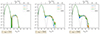 |
Fig. 7. Velocity distribution functions, f(vx), of all electrons at different moments of time. The dashed gray line indicates the initial distributions. Different lines (0, 1, 2) corresponding to particles in the areas are indicated as 0, 1 and 2 in Figure 4. The corresponding video is available online. |
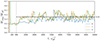 |
Fig. 8. Fraction of the beam energy that is being carried out by supra-thermal particles (with v > vT) for each diagnostic area. The dashed black line indicates the average level over the time from t = 900 |

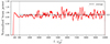 |
Fig. 9. Power of the beam at the end of the system normalised on its power at the injection moment. The dashed black line indicates the average level over the time from t = 900 |

Turning to the spectrum of oscillations in the system, according to the linear theory (Fig. 3), the most unstable mode is one with k∥ ≈ 4.3. In simulations, it is close to this value and appears to be near k∥ ≈ 4.5 at the initial stage (Fig. 10). On the non-linear stage spectrum, there are various numbers of significant modes with wave numbers up to k∥ = 7. In Fig. 12, the (ω, k∥) spectrum over the entire simulation time is presented. Aside from the plasma oscillations near the plasma frequency, there is a noticeable amount for the second harmonic and evidence for the third one, but higher modes are not visible. According to the (ω, x) spectrum (Fig. 11), all high modes of plasma oscillations are localised in area 1, mainly near x = 10 c/ωp0, where the amplitude of plasma waves are the highest and non-linear processes are the most intensive (see Fig. 5). In addition to plasma oscillations, we can see ion acoustic waves with a wide spectrum as well as a small number of EM waves in the Bz spectrum.
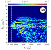 |
Fig. 10. Spectrum of the longitudinal electric field, Ex, over the simulation time. The horizontal pink line indicates a prediction of the linear theory. The vertical white line marks the time moment |

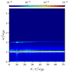 |
Fig. 11. Spectrum of plasma oscillations over the system length. |
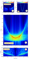 |
Fig. 12. Spectrum Bz(ω, k∥) (top right) and Ex(ω, k∥) (others) over the entire simulation time and along the entire length of the system. The vertical red lines correspond to ω = |k|⋅vb. |
4. Discussion and conclusion
The present simulation in the open boundary model with a continuously injected beam shows a higher number of supra-thermal particles appearing than in the model of infinite plasma. During the propagation through the plasma slab, beam particles lose on average 10% of their energy. We also can see some time moments when beam particles, on the contrary, increase their average energy up to 125% of the initial value. However, the most important results are the following. For the considered relative beam density, nb/n0 = 5 ⋅ 10−4, we see that the relaxation length appears to be only several dozens of c/ωp0. Within this length, the level of beam-plasma instability is high enough to be followed by modulation instability and plasma wave capturing in the density wells. After passing through this distance, the electron beam distribution function appears to be almost flat-topped. Such a beam becomes stable against two-stream instability and passes forward without significant changes.
These results show the importance of using a realistic numerical model with open boundaries and a continuously injected beam when investigating beam-plasma systems in space conditions. However, to accurately reproduce the actual level of plasma turbulence in the solar wind, the relative density of the beam should be reduced by one or two orders of magnitude. Although the use of this model is more computationally demanding than the infinite plasma one, modern computational systems are sufficient for high-resolution studies on large spatial and temporal scales.
In addition, several more approaches for realistic simulations of beam-plasma systems can be suggested. We see that after some time the system reaches some sort of steady state regime. So, instead of continuous injection of a beam, we can consider a case with a limited injection time. This would allow us to study the evolution of the waves in the system that was built up by the beam, but without beam particles. Such a problem statement is relevant for the interpretation of real beam-plasma systems, but it is impossible in the infinite plasma approximation. In the present work, the injected beam has a Maxwellian initial velocity distribution. But, as we can see from simulations, the beam distribution rapidly becomes flat-topped. So, if our goal, for example, is to investigate solar radio bursts at a significant distance from the acceleration site, then we can simulate the injection of a beam with a flat-topped VDF. This allows us to investigate the influence of realistic regular and random gradients of plasma density and the external magnetic field on beam-plasma instability, which is necessary for the appearance of plasma emission mechanisms. On the other hand, if we are mainly interested in the evolution of a beam’s VDF over a long propagation distance, then it seems appropriate to use the model of a moving frame. In such a model, we can start from an electron beam with the initial distribution on a generation site (e.g. near the Sun) and investigate its evolution during the propagation through the solar plasma, taking into account all variations of external parameters (background plasma density and magnetic field). Nowadays, this model is mainly used for plasma accelerators (Vay 2020) with a frame length of several plasma lengths. As we can see from the present simulations, for solar plasma systems with low density beams, this length should be significantly (probably hundreds of times) longer. This is necessary to develop main beam-plasma instability at the time of beam propagation. Because of the significant demand for computational resources, most likely only 1D simulations using this model are possible nowadays. However, the result of such simulations should provide an unprecedented possibility for a direct comparison with the satellite measurements of beam VDFs.
Movies
Movie 1 Access here
Movie 2 Access here
Data availability
Movies associated to Figs. 4 and 7 are available at https://www.aanda.org
Acknowledgments
The work was supported by the Ministry of Science and Higher Education of the Russian Federation. The author would like to thank Irkutsk Supercomputer Center of SB RAS for providing the access to HPC-cluster “Akademik V.M. Matrosov”.
References
- Akhiezer, A. I., & Fainberg, Y. B. 1949, Dokl. Akad. Nauk USSR, 69, 555 [Google Scholar]
- Annenkov, V., & Volchok, E. 2023, Adv. Space Res., 71, 1948 [NASA ADS] [CrossRef] [Google Scholar]
- Annenkov, V. V., Timofeev, I. V., & Volchok, E. P. 2016a, Phys. Plasmas, 23, 053101 [NASA ADS] [CrossRef] [Google Scholar]
- Annenkov, V. V., Volchok, E. P., & Timofeev, I. V. 2016b, Plasma Phys. Control. Fusion, 58, 045009 [CrossRef] [Google Scholar]
- Annenkov, V. V., Berendeev, E. A., Timofeev, I. V., & Volchok, E. P. 2018, Phys. Plasmas, 25, 113110 [NASA ADS] [CrossRef] [Google Scholar]
- Annenkov, V. V., Timofeev, I. V., & Volchok, E. P. 2019, Phys. Plasmas, 26, 063104 [Google Scholar]
- Annenkov, V. V., Volchok, E. P., & Timofeev, I. V. 2020, ApJ, 904, 88 [NASA ADS] [CrossRef] [Google Scholar]
- Annenkov, V., Volchok, E., & Timofeev, I. 2021, 47th EPS Conference on Plasma Physics, EPS 2021, 2021-June, 125 [Google Scholar]
- Annenkov, V. V., Volchok, E. P., & Timofeev, I. V. 2024, Phys. Plasmas, 31, 033104 [Google Scholar]
- Arber, T. D., Bennett, K., Brady, C. S., et al. 2015, Plasma Phys. Control. Fusion, 57, 113001 [Google Scholar]
- Arzhannikov, A. V., Ivanov, I. A., Kasatov, A. A., et al. 2020, Plasma Phys. Control. Fusion, 62, 045002 [CrossRef] [Google Scholar]
- Aschwanden, M. J. 2002, Space Sci. Rev., 101, 1 [Google Scholar]
- Bohm, D., & Gross, E. P. 1949, Phys. Rev., 75, 1864 [NASA ADS] [CrossRef] [Google Scholar]
- Boris, J. P. 1970, in Proceeding of Fourth Conference on Numerical Simulations of Plasmas (Washington D. C.: Naval Research Laboratory), 3 [Google Scholar]
- Bret, A., Gremillet, L., Bénisti, D., & Lefebvre, E. 2008, Phys. Rev. Lett., 100, 205008 [NASA ADS] [CrossRef] [Google Scholar]
- Büchner, J., Dum, C. T., & Scholer, M. 2003, in Space Plasma Simulation, eds. J. Büchner, M. Scholer, & C. T. Dum (Berlin, Heidelberg: Springer), Lect. Notes Phys., 615, 351 [Google Scholar]
- Burdakov, A., Azhannikov, A., Astrelin, V., et al. 2007, Fusion Sci. Technol., 51, 106 [Google Scholar]
- Dawson, J. M. 1983, Rev. Mod. Phys., 55, 403 [CrossRef] [Google Scholar]
- Esirkepov, T. 2001, Comp. Phys. Commun., 135, 144 [NASA ADS] [CrossRef] [Google Scholar]
- Ginzburg, V. L., & Zheleznyakov, V. V. 1958, Sov. Astron., 2, 653 [NASA ADS] [Google Scholar]
- Hapgood, M. 2016, Space Weather (IOP Publishing) [CrossRef] [Google Scholar]
- Henri, P., Sgattoni, A., Briand, C., Amiranoff, F., & Riconda, C. 2019, J. Geophys. Res.: Space Phys., 124, 2018JA025707 [Google Scholar]
- Jebaraj, I. C., Dresing, N., Krasnoselskikh, V., et al. 2023, A&A, 680, A7 [Google Scholar]
- Khotyaintsev, Y. V., Graham, D. B., Norgren, C., & Vaivads, A. 2019, Front. Astron. Space Sci., 6, 1 [Google Scholar]
- Klein, K.-L., Krucker, S., Trottet, G., & Hoang, S. 2005, A&A, 431, 1047 [NASA ADS] [CrossRef] [EDP Sciences] [Google Scholar]
- Krafft, C., & Savoini, P. 2021, ApJ, 917, L23 [NASA ADS] [CrossRef] [Google Scholar]
- Krafft, C., & Savoini, P. 2022, ApJ, 924, L24 [NASA ADS] [CrossRef] [Google Scholar]
- Krafft, C., & Savoini, P. 2023, ApJ, 949, 24 [NASA ADS] [CrossRef] [Google Scholar]
- Krafft, C., & Savoini, P. 2024, ApJ, 964, L30 [NASA ADS] [CrossRef] [Google Scholar]
- Kumar, M., Kang, T., Song, H. S., & Hur, M. S. 2022, Phys. Plasmas, 29, 033102 [Google Scholar]
- Li, C., Chen, Y., Zhang, Z., Ning, H., & Li, T. 2024, ApJ, 960, 111 [NASA ADS] [CrossRef] [Google Scholar]
- Lindholm, E., Nickolls, J., Oberman, S., & Montrym, J. 2008, in IEEE Micro, 28, 39 [CrossRef] [Google Scholar]
- Lizunov, G., Volokitin, A., & Blazhko, I. 2002, Adv. Space Res., 29, 1391 [NASA ADS] [CrossRef] [Google Scholar]
- Mandrake, L., Pritchett, P. L., & Coroniti, F. V. 2000, Geophys. Res. Lett., 27, 2869 [NASA ADS] [CrossRef] [Google Scholar]
- Melrose, D. B. 1980, Space Sci. Rev., 26, 3 [NASA ADS] [CrossRef] [Google Scholar]
- Nishikawa, K., Meli, A., Köhn, C., et al. 2023, Proc. Int. Astron. Union, 17, 44 [Google Scholar]
- Reid, H. A. S., & Ratcliffe, H. 2014, Res. Astron. Astrophys., 14, 773 [Google Scholar]
- Robinson, P. A., & Cairns, I. H. 2000, in Geophysical Monograph Series (Blackwell Publishing Ltd), 119, 37 [Google Scholar]
- Schönlein, A., Boutoux, G., Pikuz, S., et al. 2016, EPL, 114, 45002 [CrossRef] [EDP Sciences] [Google Scholar]
- Soldatkina, E., Pinzhenin, E., Korobeynikova, O., et al. 2022, Nucl. Fusion, 62, 066034 [Google Scholar]
- Spitkovsky, A. 2005, in AIP Conference Proceedings (AIP Publishing), 345 [NASA ADS] [CrossRef] [Google Scholar]
- Thornhill, S. G., & ter Haar, D. 1978, Phys. Rep., 43, 43 [Google Scholar]
- Thurgood, J. O., & Tsiklauri, D. 2016, J. Plasma Phys., 82, 905820604 [Google Scholar]
- Timofeev, I. V., Volchok, E. P., & Annenkov, V. V. 2016, Phys. Plasmas, 23, 083119 [NASA ADS] [CrossRef] [Google Scholar]
- Timofeev, I., Annenkov, V., Volchok, E., & Glinskiy, V. 2022, Nucl. Fusion, 62, 066033 [Google Scholar]
- Vay, J. L. 2020, Proceedings of the 2019 CERN–Accelerator–School Course, 21 [Google Scholar]
- Vedenov, A. A., & Rudakov, L. I. 1964, Dokl. Akad. Nauk USSR, 159, 767 [Google Scholar]
- Yee, K. S. 1966, IEEE Trans. Antennas Propag., 14, 302 [CrossRef] [Google Scholar]
- Zakharov, V. E. 1972, Sov. Phys. JETP, 35, 908 [NASA ADS] [Google Scholar]
- Zhang, Z., Chen, Y., Ni, S., et al. 2022, ApJ, 939, 63 [NASA ADS] [CrossRef] [Google Scholar]
Appendix A: The conversion factors
The conversion factors from dimensionless to dimensional units for various densities are presented in Fig. A.1. By choosing the background plasma density we determine unambiguously all parameters in the simulations. This makes it possible to apply the results obtained in the simulations to various physical systems for which the collisionless plasma approximation is applicable.
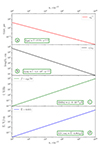 |
Fig. A.1. Correspondence between dimensional and dimensionless quantities on a logarithmic scale. a) The unit of time |

All Figures
|
Fig. 1. Schematic representation of a simulation box for infinite plasma. The cyan arrow indicates the path of one particle, which passes through all periodic boundaries. |
| In the text | |
|
Fig. 2. Simulation box with open boundaries in the longitudinal direction (x axis) and periodic boundaries in the transverse one (y axis). Beam particles are injected into the system through the left edge. They cause a return current of plasma electrons and leave the system through the right border. The flux of all of the plasma particles is maintained in a self-consistent manner on both sides. |
| In the text | |
|
Fig. 3. a) Growth rate map for the beam-plasma instability, Γ(k∥, k⊥). The green line, k⊥ = k⊥(k∥), marks the local maximal growth rate. b) Growth rate for longitudinal modes, Γ(k∥, 0). c) Growth rate on the line of the maximum, Γ(k⊥). |
| In the text | |
|
Fig. 4. Simulation results at several moments in time. Top: Density of the ions (red line), different phases of one plasma oscillation (blue lines). Bottom: Phase space, f(vx, x), of the beam. The corresponding video is available online. |
| In the text | |
|
Fig. 5. Top: Evolution of the field, Ex, maximum in space and time. Bottom: Time dependence of the field, Ex, maximum (blue) and its position (brown). The horizontal blue line marks the average value of the longitudinal electric field, Ex, in the plasma wave during the non-linear stage. |
| In the text | |
|
Fig. 6. Dependence of the instability growth rate, Γ, on time. The horizontal solid black line indicates a prediction of the linear theory. |
| In the text | |
|
Fig. 7. Velocity distribution functions, f(vx), of all electrons at different moments of time. The dashed gray line indicates the initial distributions. Different lines (0, 1, 2) corresponding to particles in the areas are indicated as 0, 1 and 2 in Figure 4. The corresponding video is available online. |
| In the text | |
|
Fig. 8. Fraction of the beam energy that is being carried out by supra-thermal particles (with v > vT) for each diagnostic area. The dashed black line indicates the average level over the time from t = 900 |
| In the text | |
|
Fig. 9. Power of the beam at the end of the system normalised on its power at the injection moment. The dashed black line indicates the average level over the time from t = 900 |
| In the text | |
|
Fig. 10. Spectrum of the longitudinal electric field, Ex, over the simulation time. The horizontal pink line indicates a prediction of the linear theory. The vertical white line marks the time moment |
| In the text | |
|
Fig. 11. Spectrum of plasma oscillations over the system length. |
| In the text | |
|
Fig. 12. Spectrum Bz(ω, k∥) (top right) and Ex(ω, k∥) (others) over the entire simulation time and along the entire length of the system. The vertical red lines correspond to ω = |k|⋅vb. |
| In the text | |
|
Fig. A.1. Correspondence between dimensional and dimensionless quantities on a logarithmic scale. a) The unit of time |
| In the text | |
Current usage metrics show cumulative count of Article Views (full-text article views including HTML views, PDF and ePub downloads, according to the available data) and Abstracts Views on Vision4Press platform.
Data correspond to usage on the plateform after 2015. The current usage metrics is available 48-96 hours after online publication and is updated daily on week days.
Initial download of the metrics may take a while.