| Issue |
A&A
Volume 584, December 2015
|
|
|---|---|---|
| Article Number | A93 | |
| Number of page(s) | 23 | |
| Section | Interstellar and circumstellar matter | |
| DOI | https://doi.org/10.1051/0004-6361/201423788 | |
| Published online | 26 November 2015 | |
Online material
Appendix A: Alternative data analysis
To investigate the robustness of the results to details of the data reduction, we calculated a set of alternative τ(250 μm) maps. In addition to the analysis of three or four Herschel bands (see Sect. 2.2), we considered the use of local background subtraction and the possibility of making a correction for residual mapping artefacts with the help of other all-sky surveys. The resulting τ(250 μm) /τ(J) ratios were compared to the values found in Sect. 3.1. The comparison was carried out without bias corrections, comparing the results with the 160−500 μm fits of Sect. 2.4.
Appendix A.1: Local background subtraction
Our default analysis is based on Herschel data for which the absolute zero points were derived from a comparison with Planck and IRAS maps. As an alternative, we used Herschel surface brightness maps from which the diffuse background was subtracted using the reference regions listed in Table 1. Thus, the average surface brightness of the reference region was subtracted from each Herschel surface brightness map separately, before calculating the colour temperatures and the dust optical depths.
The local background subtraction might be a more reliable way to ensure a consistent zero level for the compared quantities. However, it also means that colour temperature and column density can only be estimated in the part of the map in which the surface brightness values are significantly higher than those of the reference area. We masked the area in which the signal is lower than twice the estimated statistical uncertainty of the surface brightness in each band. The final mask is a combination of these masks and the original mask that eliminated the map boundaries for which the convolution to the resolution of the τ(J) data is only poorly defined.
Appendix A.2: Checks for mapping artefacts
Although Herschel data are usually of very good quality, there can still be some small artefacts that affect some parts of the maps. Errors might result from data reduction or from instrumental effects such as striping or general gain changes (Xu et al. 2014; Paladini et al. 2013). If processing includes high-pass filtering, the large-scale surface brightness gradients may be affected and the contrast between faint and bright regions may be decreased. Our maps often contain significant emission up to the map boundary. Without a flat border region with very low emission, it is difficult to estimate whether the baseline assumed for the scans is correct. Such effects could be more important and more difficult to detect for small maps. Thus, this could mostly affect PACS maps, for which the signal-to-noise ratio is also typically lower than in the SPIRE data (Juvela et al. 2010).
These effects were investigated with the help of independent FIR and submillimetre data. At 100 μm, 350 μm, and 500 μm we can compare Herschel data almost directly with the corresponding IRIS and Planck bands. The Planck 545 GHz data were corrected to 500 μm using a modified black body with the Herschel colour temperature map and β equal to 2.0. Keeping the other parameter constant, an error of 2 K in temperature or an error of 0.2 in β would both correspond to only a ~2% error in the extrapolated value. At 160 μm and 250 μm we used values interpolated from IRIS 100 μm, AKARI 140 μm (Murakami et al. 2007), and Planck 350 μm channels. Here Δβ ~ 0.2 translates into a change of less than 1% at 160 μm. For a direct extrapolation from the 350 μm to 160 μm, an error of Δβ = 0.1 would result in an error in the interpolated value that is still lower than 8%. Typically interpolation errors should thus be below the statistical errors. The same considerations apply to the zero-point corrections of Sect 2.2.2, with the difference that they are not affected by any multiplicative errors.
The reference data were compared with the original Herschel maps at 6′ resolution to derive an additive correction that leaves the median value of the maps unchanged and only affects scales larger than ~ 6′. We also checked similar multiplicative corrections, assuming that the zero points of the different surveys are compatible, and even calculating corrections where linear fits between Herschel and reference data were first used to estimate the differences in zero-point and gain calibration. The last alternative would avoid the assumptions of consistent calibration and zero points between the data sets. In most cases, there are no significant differences between the three choices. A typical map has no clear artefacts, and the proposed correction will probably decrease the data quality. However, when the local artefacts are clear (e.g., excessive surface brightness some corner of a Herschel map), the corrected map should give a better description of the true surface brightness. Thus, we do not believe that the corrected maps represent a clear improvement, but the difference between the corrected and uncorrected data should give some idea of the potential effect that artefacts of that magnitude could have.
Appendix A.3: Comparison of the data sets
We compared the τ(250 μm) /τ(J) values (without bias corrections) among six data sets: (1) three bands at 250-500 μm (our default data set); (2) four bands at 160–500 μm; (3) three bands with local background subtraction; (4) three bands with the corrections of Sect. A.2; and (5) four bands with the corrections of Sect. A.2. Table A.1 shows the results, comparing the dispersion of the obtained τ(250 μm) /τ(J) values between fields and the change in the values compared to the default case where three bands and the absolute zero points were used.
Comparison of the mean values of τ(250 μm) /τ(J) obtained with different versions of Herschel data, without bias corrections.
|
Fig. B.1
Field G300.86-9.00 as an example of τ(J) bias maps estimated with simulated NICER observations. The frames show the optical depth derived from actual observations (frame a)), average recovered extinction map in simulations (frame b)), and the bias as the difference between the output and input maps in the simulation (frame c)). |
|
| Open with DEXTER | |
The second column of the table lists the number of fields where the formal error of the slope τ(250 μm) /τ(J) is lower than 10%. This number is smaller when PACS data are included, 82–83 fields compared to the 102−105 fields with SPIRE data alone. The numbers do not include the Witch Head Nebula, for which we have no PACS data and which therefore was excluded from this comparison. The background subtraction and the Sect. A.2 corrections both decrease the mean value, but not significantly. Note that on physical grounds one could have expected the values to increase with background subtraction (if dense material has higher τ(250 μm) /τ(J)) and to decrease with the inclusion of 160 μm channel (if the inclusion of shorter wavelengths increases estimated colour temperatures). The last column shows the difference relative to our default case. In this column we only list the common set of 81 fields where the error estimates are lower than 10% for all the five cases. On average, the changes in the τ(250 μm) /τ(J) values are less than 1.0 units (lower than 5%). The dispersion between different SPIRE analyses is lower than 2.0 units and somewhat higher when analyses of four and three bands are compared.
Appendix B: Simulated NIR extinction maps
In addition to photometric errors, the reliability of NIR optical depth estimates is mainly affected by the sampling provided by the background stars and the possible contamination by foreground stars and galaxies.
We used 2MASS catalogue flags to eliminate most of the obvious galaxies. In addition to requiring a photometric quality corresponding to ph_qual in classes A–C, we excluded all point sources that were extended (flag ext_key is set) or were flagged with gal_contam. These only remove part of the galaxies. The increased dispersion of intrinsic colours caused by galaxies is taken into account in the error estimates provided by the method NICER. Because our simulations use actual 2MASS data near the target fields, this extragalactic contamination is also automatically present in the simulations described below.
The simulations are based on dust 250 μm optical depth maps derived from Herschel observations. Using only SPIRE data, we derive column densities at 25″ resolution as a combination of ![]() (B.1)where τ(500) is calculated using 250, 350, and 500 μm maps at the lowest common resolution, τ(350) is calculated similarly from 250 μm and 350 μm maps, and τ(350 → 500) is the latter convolved to the resolution of the 500 μm observations (see Palmeirim et al. 2013). Thus, the expression in square brackets describes structures that are seen at the resolution of 350 μm data (25″), but not at the resolution of 500 μm data (36″). The calculations assume a fixed value β = 2.0. The differences to the τ(250 μm) maps used in Sect. 3 are small and, furthermore, we only consider differences between these input maps and the values recovered by NICER. On the other hand, we wish to retain the highest resolution possible (18″ instead of 36″) because the bias in NICER estimates is probably linked to the amount of small-scale structure.
(B.1)where τ(500) is calculated using 250, 350, and 500 μm maps at the lowest common resolution, τ(350) is calculated similarly from 250 μm and 350 μm maps, and τ(350 → 500) is the latter convolved to the resolution of the 500 μm observations (see Palmeirim et al. 2013). Thus, the expression in square brackets describes structures that are seen at the resolution of 350 μm data (25″), but not at the resolution of 500 μm data (36″). The calculations assume a fixed value β = 2.0. The differences to the τ(250 μm) maps used in Sect. 3 are small and, furthermore, we only consider differences between these input maps and the values recovered by NICER. On the other hand, we wish to retain the highest resolution possible (18″ instead of 36″) because the bias in NICER estimates is probably linked to the amount of small-scale structure.
The Besancon model (Robin et al. 2003) was used to create a simulated catalogue of stars over a 0.5° × 0.5° area centred on each target field. The catalogue includes stellar distances and H-band magnitudes, and together with the distance estimates listed in Table 1, this was converted into the probability that a star of given magnitude resides between the cloud and the observer. In the simulation, the corresponding fraction of stars was assumed to be located in front of the cloud.
To simulate NIR observations, we used the same 2MASS data that were used to calculate the actual τ(J) maps of the fields. The stars in the reference area (see Table E.1) were used to determine an empirical probability distribution of H-band magnitudes and the dependence between the J, H, and Ks magnitudes and their uncertainties, as given in the 2MASS catalogue. This reference area may be affected by small amounts of absorption by diffuse dust, but gives a good approximation of the brightness distribution of stars that are unextincted by the main cloud.
We simulated a uniform distribution of stars over the Herschel field, generating the magnitudes from the empirical H-band magnitude distribution and matching the average stellar density of the reference region. The J and Ks magnitudes of each star were generated using the J−H and H−Ks colours of a random star selected from the reference region. This ensures that the distribution of intrinsic colours is realistic and that the simulations reproduce proper correlations (also in errors) between the bands.
Based on the Besancon model, a fraction of stars was assumed to reside in front of the cloud and to be unaffected by extinction. For the remaining stars, the line-of-sight optical depth in J band was calculated using the input column density map and a fixed ratio of τ(250 μm) /τ(J) = 1.5 × 10⁻³. The optical depths in H and Ks bands then follow from the Cardelli et al. (1989) extinction curve. The magnitudes were adjusted according to the line-of-sight optical depths. The magnitudes and their uncertainties in the reference area were used to calculate the typical photometric uncertainties as a function of magnitude, and they were used in the NICER calculation. Because the intrinsic colours of the stars were generated based on observed stars, no additional scatter needed to be added for intrinsic colours. However, because the extinction makes the stars fainter, the typical photometric errors increase as well. This was taken into account by adding normal distributed noise to the magnitudes, which corresponds to the difference in the typical uncertainties between the original and the extincted magnitudes.
The simulated stellar catalogues were fed to the NICER algorithm to derive extinction maps with the same parameters as in Sect. 2.3. For each target field, one hundred realisations of the τ(J) maps were calculated to obtain maps for the standard deviation and the bias of the estimated τ(J) values. Figure B.1 shows one example.
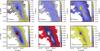 |
Fig. C.1
Field G300.86-9.00 as an example of the τ(250 μm) bias estimation with radiative transfer modelling. Upper row: relative error between the model predicted surface brightness and the observations at 250 μm, 350 μm, and 500 μm. Lower frames: colour temperature and τ(250 μm) maps calculated from the synthetic observations and the relative bias in τ(250 μm) obtained by comparison with the actual τ(250 μm) values in the model. |
| Open with DEXTER | |
Appendix C: Simulated Herschel observations
The estimation of the τ(250 μm) bias is more uncertain than the estimation of τ(J) bias. Because of line-of-sight temperature variations, the colour temperature overestimates the mass-averaged dust temperature, which translates into too low estimates of τ(250 μm). The magnitude of the effect cannot be estimated precisely because the line-of-sight temperature distribution is unknown. Order of magnitude estimates can be obtained with radiative transfer modelling by making assumptions of the radiation field, dust properties, and the cloud structure.
We carried out radiative transfer calculations individually for all the 116 fields. We assumed constant dust properties corresponding to Milky Way dust with a selective extinction of RV = 5.5 (Draine 2003b). The initial radiation field was assumed to correspond to the Mathis et al. (1983) model of solar neighbourhood. The spectrum of the illuminating radiation has an impact on the temperature contrasts. We have no way to independently determine the shape of the spectrum of the radiation field. However, this typically remains a second-order effect, and the main effect, the level of the radiation field intensity, is part of the modelling. One exception are the possible stars that heat clouds from the inside and may locally have a strong effect. These are considered later in the analysis, but are not part of the simulations.
For each field, we built a model that attempts to reproduce the 250–500 μm observations of that field. From the background-subtracted surface brightness maps we selected the central 30′ × 30′ area. The model cloud had the same angular dimensions and was discretised onto a 1813 cell grid. Each cell of the model therefore corresponds to an angular size of 10″, but the linear scale depends on the distance of the cloud. In the line-of-sight direction we assumed a Gaussian density distribution with a FWHM equal to 25% of the field size. The linear size again depends on the cloud distance because in more distant fields we are also probably concerned with larger structures. In the line-of-sight direction the density peak is always in the central plane of the model cube. This increases mutual shadowing of dense regions, which in reality can reside at different distances and increases the temperature contrasts in the model. On the other hand, for a field at 200 pc distance, the selected line-of-sight FWHM extent is ~0.4 pc, which is larger than the size of typical cores. Therefore, it is difficult to say whether the selection of this particular line-of-sight density profile leads to an over- or underestimation of the final τ(250 μm) bias. These are usually second-order effects (Juvela et al. 2013) except for very dense clumps that can remain practically invisible in τ(J) maps as well.
We carried out radiative transfer calculations to produce synthetic surface brightness maps at Herschel wavelengths that were then convolved to the resolution of the observations. The ratio of observed and modelled 350 μm maps was used to adjust the column densities, applying the same multiplicative factor to all cells along the same line-of-sight. The intensity of the external radiation field was scaled based on the ratios between the observed and modelled 250 μm and 500 μm surface brightness. The aim is to also reproduce the average shape of the spectra. The full procedure was iterated until the model matched the observed 350 μm map at ~1% accuracy and the average ratio 250 μm/500 μm were correct within the same tolerance.
The final model takes into account the range of column density, the morphology, and the radiation field intensity of a field. It is not necessarily a perfect match to all surface brightness maps, but is a good facsimile of the pixel-by-pixel column density structure. We analysed the synthetic surface brightness maps as in Sect. 2.2.3. The comparison of the obtained τ(250 μm) estimates and the true values known for the model cloud gives a 30′ × 30′ map of the τ(250 μm) bias (resolution 40″). The remaining border areas usually have a low column density and therefore low bias. However, to extend bias estimates over the whole map area, we assigned values calculated using the average bias vs. column density relation estimated from central 30′ × 30′ area to the remaining pixels.
Figure C.1 shows one example, the surface brightness maps produced by the model and the bias in the τ(250 μm) values estimated from these synthetic observations.
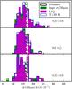 |
Fig. D.1
Comparison of Δτ(250 μm)/Δτ(J) bias-corrected distributions. In addition to the default case, derived distributions are shown for tests with larger τ(250 μm) error estimates, normal unweighted least squares, and fits excluding data affected by regions with dust temperatures exceeding 20 K. |
| Open with DEXTER | |
Appendix D: Additional checks of correlations between τ(250 μm) and τ(J)
In addition to the factors examined in Sect. 2.4, we checked the importance of two additional factors, the technical implementation of the least-squares fits, and the importance of internally heated regions.
The total least-squares fits of Sect. 2.4 used the formal error estimates of τ(J) and τ(250 μm). The former were obtained from NICER routine, the latter were estimated with MCMC calculations starting with the assumption of 7% (SPIRE) or 15% (PACS) relative errors in the surface brightness data. If the correlation is poor, the estimated slope becomes sensitive to the error estimates. For example, if the true errors of τ(250 μm) were much larger, for example because of some artefacts in map making, the use of too low error estimates would increase the slope estimates. We checked this by repeating the analysis using twice the original τ(250 μm) error estimates. In an extreme case, we can ignore the error estimates altogether and perform unweighted least-squares fits. Based on the error estimates used, the true relative uncertainty is significantly larger in τ(J) than in τ(250 μm). Therefore, the unweighted least-squares fit probably underestimates the true slope.
The third test concerns the internally heated regions in which because of strong temperature variations combined with compact, high column density clumps, both optical depth estimates are particularly uncertain. Furthermore, the estimates of τ(250 μm) bias are probably incorrect in the same areas. This is caused by two factors. First, without the internal heating source,
the models are unable to produce sufficient surface brightness values and result in very high column densities and thus high estimates of the bias (Juvela et al. 2013). Second, in the real clump the internal heating may help to decrease the actual bias if the clump centre remains warm instead of being too cold to be registered in Herschel bands (Malinen et al. 2011). We repeated the analysis of Sect. 2.4 by masking warm regions. We first masked all pixels for which the dust colour temperature was higher than 20 K. The mask was then extended to cover areas in which after convolution to 180″ resolution, the influence of the T> 20 K region was more than 10% of the convolved value.
Figure D.1 compares the result with the bias-corrected results already shown in Fig. 4. It shows that the shape of the distribution is not sensitive to the fitting procedure, nor is it significantly affected by the warm regions.
Appendix E: Maps of τ(250 μm) /τ(J) ratio
In the least-squares fits of Sect. 3.4, the interesting parameters, k and C were independent of additive errors in the correlated quantities. The highest τ(J) points were particularly important, both visually and regarding the fitted parameters. As mentioned in Sect. 3.5, we also calculated maps of the τ(250 μm) /τ(J) ratio. Because the column densities are typically low over most of the mapped area, the visual appearance of the maps is dominated by regions with low τ(250 μm) and τ(J) values where, by definition, the results become sensitive to any zero-point mismatch.
The maps were calculated by first correcting the τ(250 μm) and τ(J) maps for the bias that was estimated with modelling (see Sect. B and Sect. C). The maps of τ(250 μm) were then convolved to the resolution of the τ(J) map. A 2′ wide region near the Herschel map borders was masked because the convolved values would be affected by data outside our map coverage. Before calculating the ratio τ(250 μm) /τ(J), we subtracted from both quantities the values in the reference regions that are listed in Table 1. A typical diameter of these reference areas is ~ 6′. For τ(250 μm) the statistical error of the reference value is very small. The true uncertainty of the remaining τ(250 μm) is completely dominated by systematic errors. Because the main purpose of the ratio maps is to determine variations in the τ(250 μm) /τ(J) ratio, we are not very concerned with multiplicative errors.
We expect the statistical errors to be more significant in τ(J) and, because the variable is in the denominator, we need to mask areas with a low SN of τ(J). NICER has provided error maps for τ(J), but here we estimated the uncertainty using the following procedure: We took the data plotted in Fig. 8, selected 20% of the lowest τ(J) points, and subtracted from them the prediction of the non-linear fit (red line in Fig. 8). The uncertainty of the reference value, Δτ(J), was calculated as the standard deviation of the residuals, scaled by the ratio of (90″)2 and the area of the reference region. This should be a very conservative estimate because it assumes that in Fig. 8 the scatter would be due to τ(J) errors alone.
The results are shown in Fig. E.1. The first frames show the τ(250 μm) maps, the contours indicating the region with a SN of each parameter higher than one. The second frames show the calculated maps of τ(250 μm) /τ(J). The regions where either parameter falls below SN = 0.5 were masked. The remaining frames show the extreme cases corresponding to τ(J) ± Δτ(J) and τ(250 μm) ± δτ(250 μm), where δτ(250 μm) is the estimated error map (see Sect. 2.2.3).
 |
Fig. E.1
Maps of τ(250 μm) /τ(J) for the selected fields. Upper frames: τ(250 μm) (frame a)) and the ratio τ(250 μm) /τ(J). Lower frames: the lower (frame c)) and upper (frame d)) limits of τ(250 μm) /τ(J) calculated as (τ(250 μm) + δτ(250 μm))/(τ(J)−Δτ(J)) and (τ(250 μm)−δτ(250 μm))/(τ(J) + Δτ(J)) where δτ(250 μm) is the error map of τ(250 μm) and Δτ(J) is the estimated uncertainty of the τ(J) zero point. The areas in which the SN of either variable drops below 0.5 have been masked. In the first frame, the black contour corresponds to τ(250 μm) = δτ(250 μm) and the dashed white contour to τ(J) = Δτ(J). |
| Open with DEXTER | |
© ESO, 2015
Current usage metrics show cumulative count of Article Views (full-text article views including HTML views, PDF and ePub downloads, according to the available data) and Abstracts Views on Vision4Press platform.
Data correspond to usage on the plateform after 2015. The current usage metrics is available 48-96 hours after online publication and is updated daily on week days.
Initial download of the metrics may take a while.