| Issue |
A&A
Volume 580, August 2015
|
|
|---|---|---|
| Article Number | A142 | |
| Number of page(s) | 30 | |
| Section | Stellar structure and evolution | |
| DOI | https://doi.org/10.1051/0004-6361/201424592 | |
| Published online | 21 August 2015 | |
Online material
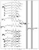 |
Fig. 7
Sequence of the observed late-time (day 100−415) spectra for SN 2011dh. Spectra obtained on the same night using the same telescope and instrument have been combined and each spectra have been labelled with the phase of the SN. Telluric absorption bands are marked with a ⊕ symbol in the optical and are shown as grey regions in the NIR. |
| Open with DEXTER | |
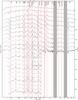 |
Fig. 8
Optical and NIR (interpolated) spectral evolution between days 5 and 425 for SN 2011dh with a 20-day sampling, where most of the lines identified in J14 have been marked with red dashed lines. Telluric absorption bands are marked with a ⊕ symbol in the optical and are shown as grey regions in the NIR. |
| Open with DEXTER | |
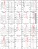 |
Fig. 9
The (interpolated) spectral evolution after day 100 for most of the lines identified in J14. Multiple or blended lines are marked with red dashed lines and telluric absorption bands in the NIR are shown as grey regions. |
| Open with DEXTER | |
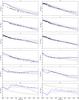 |
Fig. 17
Observed (black circles) and J14 model optical, NIR, and MIR (absolute) magnitudes between days 100 and 500 normalized to the radioactive decay chain luminosity of 0.075 M⊙ of 56Ni. The preferred model (12F) is shown as a blue solid line. The other models are shown in shaded colour as follows: 12A (red solid line), 12B (green solid line), 12C (magenta solid line), 12D (yellow solid line), 12E (cyan solid line), 13A (red short-dashed line), 13C (yellow short-dashed line), 13D (cyan short-dashed line), 13E (magenta short-dashed line), 13G (blue short-dashed line), 17A (blue long-dashed line). |
| Open with DEXTER | |
Late-time (after day 100) optical colour-corrected JC U and S-corrected JC BVRI magnitudes for SN 2011dh.
Late-time (after day 100) optical colour-corrected SDSS u and S-corrected SDSS griz magnitudes for SN 2011dh.
Late-time (after day 100) NIR S-corrected 2MASS JHK magnitudes for SN 2011dh.
Late-time (after day 100) MIR Spitzer S1 and S2 magnitudes for SN 2011dh.
List of late-time (after day 100) optical and NIR spectroscopic observations.
Pseudo-bolometric UV-to-MIR lightcurve between days 3 and 400 for SN 2011dh calculated from spectroscopic and photometric data with a 1-day sampling between days 3 and 50 and a 5-day sampling between days 50 and 400.
Appendix A: Data reductions and calibration
Template subtraction.
The optical and NIR images obtained between days 100 and 500 have been template subtracted after day 300, before which comparison of photometry on original and template subtracted images shows that the background contamination is negligible. The optical templates were constructed by point spread function (PSF) subtraction of the SN from observations acquired after day 600, and the NIR templates by PSF subtraction of the SN from the day 339 WHT observation, which is of excellent quality. For the last day 380 WHT observation we used PSF photometry.
S-corrections.
The optical and NIR photometry between days 100 and 500 have been S-corrected, and the accuracy of the photometry depends critically on the accuracy of these corrections. Figure A.1 shows the difference between colour and S-corrections for the Johnson-Cousins (JC) and 2 Micron All Sky Survey (2MASS) systems for most telescope/instrument combinations used, and S-corrections are clearly necessary for accurate photometry. In some cases, e.g. for the CA-2.2 m/CAFOS and NOT/ALFOSC I band and the CA-3.5 m/O2000 J band, the differences become as large as 0.3−0.5 mag. In particular, the difference between the NOT/ALFOSC and CA-2.2 m/CAFOS I-band observations are ~0.8 mag at day ~250, mainly because of the strong [Ca ii] 7291, 7323 Å and Ca ii 8498, 8542, 8662 Å lines. As the spectral NIR coverage ends at day ~200, we have assumed that the 2MASS S-corrections do not change after this epoch. This adds uncertainty to the 2MASS photometry after day ~200, but as the 2MASS S-corrections, except for the CA-3.5 m/O2000 J band, are generally small and evolve slowly, the errors arising from this approximation are probably modest. The accuracy of the S-corrections can be estimated by comparing S-corrected photometry obtained with different telescope/instrument combinations. The late-time JC and Sloan Digital Sky Survey (SDSS) photometry were mainly obtained with the NOT, but comparisons between S-corrected NOT/ALFOSC, LT/RATCam and CA-2.2 m/CAFOS photometry at ~300 days, show differences at the 5 per cent level, suggesting that the precision from the period before day 100 is maintained (E14). The late-time 2MASS photometry was obtained with a number of different telescopes, and although the sampling is sparse, the shape of the lightcurves suggests that the errors in the S-corrections are modest. Additional filter response functions for AT and UKIRT have been constructed as outlined in E14.
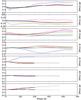 |
Fig. A.1
Difference between JC BVRI colour and S-corrections for NOT/ALFOSC (black), LT/RATCam (red), CA-2.2 m/CAFOS (blue), TNG/LRS (green), AS-1.82 m/AFOSC (yellow), and AS-Schmidt (magenta), and difference between 2MASS JHK colour and S-corrections for NOT/NOTCAM (black), TCS/CAIN (red), CA-3.5 m/O2000 (blue), TNG/NICS (green), WHT/LIRIS (yellow), and UKIRT/WFCAM (magenta). Results based on extrapolated 2MASS S-corrections are shown as dotted lines. |
| Open with DEXTER | |
Observations after day 600.
The results for the observations obtained after day 600 have been adopted from the pre-explosion difference imaging presented in E14, assuming that the remaining flux at the position of the progenitor originates solely from the SN. The observations were S-corrected using the day 678 spectrum of SN 2011dh (Shivvers et al. 2013). Comparing to results from PSF photometry, where we iteratively fitted the PSF subtracted background, we find differences of ≲0.1 mag. Given that the pre-explosion magnitudes (which were measured with PSF photometry) are correctly measured, the difference-based magnitudes are likely to have less uncertainty. On the other hand, the PSF photometry does not depend on the the pre-explosion magnitudes. The good agreement found using these two, partly independent methods gives confidence in the results. Further confidence is gained by comparing the S-corrected NOT and HST (Van Dyk et al. 2013) V-band observations, for which we find a difference of ≲0.2 mag. The assumption that the flux at the position of the progenitor originates solely from the SN, is supported by the the depth of absorption features and the line dominated nature of the day 678 spectrum.
Spitzer Telescope observations.
For the photometry after day 100 we used a small aperture with a 3 pixel radius, and a correction to the standard aperture given in the IRAC Instrument Handbook determined from the images. All images were template subtracted using archival images as described in (E14). After day 100, background contamination becomes important, and template subtraction is necessary to obtain precision in the photometry. The photometry before day 700 previously published by Helou et al. (2013) agrees very well with our photometry, the differences being mostly ≲5 per cent.
Appendix B: Line measurements
Line emitting regions.
To estimate the sizes of the line emitting regions, we fit the line profile of a spherically symmetric region of constant line emissivity, optically thin in the line (no line scattering contribution) and with a constant absorptive continuum opacity, to the observed, continuum subtracted line profile (see below). The fitting is done by an automated least-square based algorithm, and the method gives a rough estimate of the size of the region responsible for the bulk of the line emission. The absorptive continuum opacity is included to mimic blue-shifts caused by obscuration of receding-side emission. Some lines arise as a blend of more than one line, which has to be taken into account. The [O i] 6300 Å flux was calculated by iterative subtraction of the [O i] 6364 Å flux, from the left to the right, using F6300(λ) = F6300,6364(λ)−F6300(λ−Δλ) /R, where Δλ is the wavelength separation between the [O i] 6300 Å and 6364 Å lines and R the [O i] 6300, 6364 Å line ratio. This ratio was assumed to be 3, as is supported by the preferred J14 steady-state NLTE model and estimates based on small scale fluctuations in the line profiles (Sect. 3.6). For all other blended lines, we make a simultaneous fit with the line ratios as free parameters, assuming a common size of the line emitting regions. When fitting the [Ca ii] 7291, 7323 Å line we exclude the region >3000 km s-1 redwards 7291 Å, which could be contaminated by the [Ni ii] 7378, 7411 Å line (J14).
Line asymmetries.
To estimate the asymmetry of a line we calculate the first wavelength moment of the flux (center of flux) for the continuum subtracted line profile (see below). The rest wavelength is assumed to be 6316 Å and 7304 Å for the [O i] 6300, 6364 Å and [Ca ii] 7291, 7323 Å lines, respectively. This is appropriate for optically thin emission if we assume the upper levels of the [Ca ii] 7291, 7323 Å line to be populated as in local thermal equilibrium (LTE). Optically thin emission for these lines is supported by the preferred J14 steady-state NLTE model, the absence of absorption features in the observed spectra and the [O i] 6300, 6364 Å line ratio (Sect. 3.6). The rest wavelength is assumed to be 5896 Å and 8662 Å for the Na i 5890, 5896 Å and Ca ii 8498, 8542, 8662 Å lines, respectively. This is appropriate for optically thick emission, where the line emission will eventually scatter in the reddest line. Optically thick emission for the Na i 5896 Å line is supported by the preferred J14 steady-state NLTE model and the observed P-Cygni profile. For the Ca ii 8662 Å line this assumption is less justified.
Continuum subtraction.
Before fitting the line emitting region or calculating the center of flux, the continuum is subtracted. The flux is determined by a linear interpolation between the minimum flux on the blue and red sides of the smoothed line profile. The search region is set to ±6000 km s-1 for most of the lines, ±10 000 km s-1 for the Ca ii 8662 Å line and ±3000 km s-1 for the [Fe ii] 7155 Å line.
Small scale fluctuations.
To remove the large scale structure from a line profile we iteratively subtract a 1000 km s-1 box average (i.e. the result of each subtraction is fed into the next one). This procedure is repeated three times, and in tests on the product of synthetic large and small scale structures, the small scale structure is recovered with reasonable accuracy. Using a Monte Carlo (MC) analogue of the Chugai (1994) model the spatial (relative) rms of the recovered small scale structure is found to agree well with the actual (relative) rms of the fluctuations (δF in Chugai 1994, Eq. (11)).
Appendix C: Steady-state NLTE modelling.
Effects of the model parameters.
To analyse the effects of the model parameters on the model lightcurves, a split into a bolometric lightcurve and a bolometric correction (BC) is convenient. In terms of these quantities, the broad-band and pseudo-bolometric7 magnitudes are given by M = MBol−BC. This split is most useful as the bolometric lightcurve depends only on the energy deposition8, whereas the BCs depend on how this energy is processed. The energy deposition is independent of molecular cooling and dust and, within the parameter space covered by the J14 models, only weakly dependent on the density contrast and the positron trapping. Therefore, the bolometric lightcurves depend significantly only on the initial mass and the macroscopic mixing, whereas the other parameters only significantly affect the BCs. Figures C.1 and C.2 show the pseudo-bolometric and broad-band BCs for the J14 models. The optical-to-MIR BCs show small differences whereas the optical and, in particular, the broad-band BCs show considerably larger differences, which makes them well suited to constrain the model parameters. We have investigated the dependence of each BC on each parameter, and in Sects. 4.1.4 and 4.1.5 we make use of these results. The bolometric lightcurves (not shown) could as well be calculated with HYDE, and their dependence on the initial mass and macroscopic mixing is better investigated with the hydrodynamical model grid.
The optical-to-MIR BC.
The optical-to-MIR BCs for the J14 models show small differences (<±0.1 mag) between days 100 and 400, which subsequently increase towards ±0.25 mag at day 500. At day 100 the optical-to-MIR BC is >−0.15 mag, which is likely to hold before day 100 as well. In Sect. 4.2, we take advantage of these facts and use the optical-to-MIR BC for the preferred J14 model for all hydrodynamical models. However, as the J14 models cover a restricted volume of parameter space as compared to the hydrodynamical model grid, we need to justify this choice further. It is reasonable to assume that the BC depends mainly on the energy deposition per unit mass (determining the heating rate) and the density (determining the cooling rate). Furthermore, we know beforehand that hydrodynamical models giving a bad fit for the period before day 100 will not give a good fit for the period before day 400. Inspecting the hydrodynamical models (for the period before day 100) with a normalized standard deviation in the fit less than 3, we find that these do not span a wide range in (mass averaged) density or energy deposition per mass, and inspecting the J14 models we find that these cover about half of this region. Although these quantities evolve quite strongly with time, they scale in a similar way for all models, and this conclusion holds from day 100 to 400. The effect of the steady-state NLTE parameters that do not map onto the hydrodynamical parameter space (dust, molecular cooling, positron trapping, and density contrast) is harder to constrain. The small spread in the BC for the J14 models between days 100 and 400, however, make this caveat less worrying.
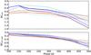 |
Fig. C.1
Optical (upper panel) and optical-to-MIR (lower panel) BCs between days 100 and 500 for the J14 models. The models are shown as in Fig. 17. |
| Open with DEXTER | |
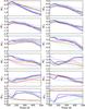 |
Fig. C.2
Broad-band BCs between days 100 and 500 for the J14 models. The models are shown as in Fig. 17. |
| Open with DEXTER | |
Treatment of molecular cooling.
Molecular cooling is included in the modelling in a simplified way, and is represented as the fraction of the (radiative and radioactive) heating emitted as molecule (CO and SiO) emission in the O/C and O/Si/S zones. The CO and SiO fundamental and first-overtone band emission is represented as box line profiles between 2.25−2.45 (CO first-overtone), 4.4−4.9 (CO fundamental), and 4.0−4.5 (SiO first-overtone) μm. The CO first-overtone band overlaps partly with the K band, and the CO fundamental and SiO first-overtone bands overlap with the S2 band, whereas the SiO fundamental band lies outside the U to S2 wavelength range. The fundamental to first-overtone band flux ratios are assumed to be the same as observed for CO in SN 1987A (Bouchet & Danziger 1993). We have used two configurations, one where the fraction of the heating emitted as molecule emission has been set to one, and one where this fraction has been set to zero. We note that CO fundamental band emission dominates the contribution to the S2 band in all models at all times. This is because the O/Si/S to O/C zone mass ratio and the CO and SiO fundamental to first-overtone band ratios are all ≲1, decreasing with increasing initial mass and with time, respectively.
Treatment of dust.
Dust is included in the modelling in a simplified way, and is represented as a grey absorptive opacity in the core. The absorbed luminosity is re-emitted as blackbody emission with a temperature determined from fits to the photometry. The dust emission is treated separately from the modelling, and is added by post-processing of the model spectra. All the models presented in J14 have the same optical depth and dust temperature, determined from the pseudo-bolometric optical lightcurve and fits to the H, K, and S1 photometry, as described below. In addition we have constructed two new models: 12E, which differs from 12C only in the absence of dust, and 12F, which differs from 12C only in the optical depth and the method used to determine the temperature.
The J14 models have an optical depth of 0.25, turned on at day 200, which approximately matches the behaviour of the optical pseudo-bolometric lightcurve. The temperature is constrained to scale as for a homologously expanding surface, representing a large number of optically thick dust clouds (J14). Minimizing the sum of squares of the relative flux differences of model and observed H, K, and S1 photometry at days 200, 300, and 400 (including H only at day 200), we find temperatures of 2000, 1097, and 668 K at days 200, 300, and 400, respectively, given the constraint Tdust< 2000 K. The S2 band was excluded as this band might have a contribution from molecule emission, whereas we know that the contribution from CO first-overtone emission to the K band at day 206 is negligible. However, the fractional area of the emitting surface (xdust), turns out to be ~20 times smaller than the fractional area needed to reproduce the optical depth, so the derived temperature is not consistent with the assumptions made.
Model 12F has an optical depth of 0.44, turned on at day 200, which better matches the behaviour of the optical pseudo-bolometric lightcurve. The constraint on the temperature evolution used for the J14 models has been abandoned, and fitting the H, K, and S1 photometry as described above, we find temperatures of 1229, 931, and 833 K at days 200, 300, and 400, respectively. This shows that, in addition to the inconsistency between the absorbing and emitting area, the scaling of temperature is not well reproduced by the J14 models. Because of the better reproduction of the optical pseudo-bolometric lightcurve and the problems with the temperature scaling used for the J14 models, we use model 12F instead of model 12C as our preferred model in this paper. Abandoning all attempts to physically explain the temperature leaves us with black box model, parametrized with the optical depth and the temperature. This is a caveat, but also fair, as the original model is not self-consistent. We note that the good spectroscopic agreement found for model 12C in J14 does not necessarily apply to model 12F. However, for lines originating from the core, which are expected to be most affected by the higher optical depth of the dust, the flux would be ~17 per cent lower and the blue-shifts ~100 km s-1 higher (Sect. 3.5), so the differences are likely to be small.
Appendix D: HYDE and the model grid
HYDE.
Is a one-dimensional Lagrangian hydrodynamical code based on the flux limited diffusion approximation, following the method described by Falk & Arnett (1977), and adopting the flux limiter given by Bersten et al. (2011). The opacity is calculated from the OPAL opacity tables (Iglesias & Rogers 1996), complemented with the low temperature opacities given by Alexander & Ferguson (1994). In addition we use an opacity floor set to 0.01 cm2 gram-1 in the hydrogen envelope and 0.025 cm2 gram-1 in the helium core, following Bersten et al. (2012, priv. comm.), who calibrated these values by comparison to the STELLA hydrodynamical code (Blinnikov et al. 1998). The electron density, needed in the equation of state, is calculated by solving the Saha equation using the same atomic data as in Jerkstrand et al. (2011, 2012). The transfer of the gamma-rays and positrons emitted in the decay chain of 56Ni is calculated with a MC method, using the same grey opacities, luminosities, and decay times as in Jerkstrand et al. (2011, 2012).
The model grid.
Is based on non-rotating solar metallicity helium cores, evolved to the verge of core-collapse with MESA STAR (Paxton et al. 2011). The configuration used was the default one, and a central density limit of 109.5 gram cm-3 was used as termination condition. The evolved models span MHe = 4.0−5.0 M⊙ in 0.25 M⊙ steps and MHe = 5.0−7.0 M⊙ in 0.5 M⊙ steps. Below 4.0 M⊙, stellar models were constructed by a scaling
of the 4.0 M⊙ density profile. The SN explosion was parametrized with the injected explosion energy (E), the mass of the 56Ni (MNi), and its distribution. The mass fraction of 56Ni (XNi) was assumed to be a linearly declining function of the ejecta mass (mej) becoming zero at some fraction of the total ejecta mass (MixNi), expressed as XNi ∝ 1−mej/ (MixNiMej), XNi ≥ 0. We note that this expression allows MixNi> 1, although the interpretation then becomes less clear. The total volume of parameter space spanned is MHe = 2.5−7.0 M⊙, E = 0.2−2.2 × 1051 erg, MNi = 0.015−0.250 M⊙, and MixNi = 0.6−1.6 using a 12 × 16 × 13 × 9 grid. A mass cut with zero velocity was set at 1.5 M⊙, and the material below is assumed to form a compact remnant, although fallback of further material onto this boundary is not prohibited. To calculate bolometric lightcurves between days 100 and 400 we run HYDE in homologous mode, ignore the radiative transfer, and take the bolometric luminosity as the deposited radioactive decay energy (Appendix C).
© ESO, 2015
Current usage metrics show cumulative count of Article Views (full-text article views including HTML views, PDF and ePub downloads, according to the available data) and Abstracts Views on Vision4Press platform.
Data correspond to usage on the plateform after 2015. The current usage metrics is available 48-96 hours after online publication and is updated daily on week days.
Initial download of the metrics may take a while.