| Issue |
A&A
Volume 575, March 2015
|
|
|---|---|---|
| Article Number | A38 | |
| Number of page(s) | 16 | |
| Section | Cosmology (including clusters of galaxies) | |
| DOI | https://doi.org/10.1051/0004-6361/201425278 | |
| Published online | 19 February 2015 | |
Online material
Appendix A: Maps, spectra, and velocity limits
We have placed the MOS 1 images, the RGS spectra, and the velocity limits in this section to unburden the paper reading.
The MOS 1 images (Fig. A.1) are obtained by stacking the Fe-L (10–14 Å) band images extracted in each exposure (see Sect. 3.3). We zoomed on the central 10′ region.
In Table A.1, we quote all our velocity results. In Fig. A.2 (left panel), we compare the 2σ upper limits on the velocity broadening as measured for the 3.4′ and 0.8′ regions by subtracting the MOS 1 spatial profiles. In Fig. A.2 (right panel), we compare the 0.8′2σ upper limits estimated by subtracting the adopted and the best-fit, spatial-line-broadening (see Sect. 4.2). In Table A.1, we also show the total line widths as result of spatial plus Doppler broadening with their 68% uncertainties. These total widths are clearly dominated by the spatial broadening.
In Table A.2, we report the values of r500 and K0 adopted with with the physical scales, the RGS temperatures estimated with an isothermal model, the conservative upper limits on the velocities and the Mach numbers, the limits separately measured for the O viii, Fe xvii, and Fe xx-to-xxiv emission lines, and finally the velocity limits for the two CIE components where it was possible to fit them separately. The separate
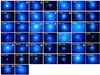 |
Fig. A.1
MOS 1 stacked Fe-L band images: Central 10′ × 10′ region. The starred clusters are part of our new campaign (see also Sect. 3.3). |
| Open with DEXTER | |
Fe xvii and 2-T fits were accessible only for a very limited sample of sources with both strong high- and low-ionization Fe lines (see Sect. 5.1). In Fig. A.3, we compare the velocity upper limits estimated with both the standard and the conservative methods with the average RGS temperature measured with an isothermal model, the sound speed, and the fractions of thermal energy stored in turbulence. In Fig. A.4 (left panel), we show the Mach number as a function of the temperature with the pointsize and, it is color coded according to the physical scale and the central entropy, respectively. The lines show the average Mach number calculated within particular ranges of physical scales. In Fig. A.4 (left panel), we show the Mach number scaled by the 1/3rd power of the physical scale, assuming Kolmogorov turbulence (see also Sect. 5.2).
In Figs. A.5−A.7, we show the RGS spectra extracted in the 3.4′ cross-dispersion region (see also Sect. 3.2). The spectra were combined with the rgscombine task for plotting purposes. We have adapted the spectral model from the bestfit obtained for the parallel modeling of the individual exposures. Most spectra were fitted with a multi-temperature, two-cie model (see Sect. 4). A few of them require just a single cie component. The spectral modeling involved the 7 − 28 Å band, but we focus on the shorter 10 − 21 Å band containing the Fe, Ne, and O lines.
|
Fig. A.2
Left panel: velocity broadening at 2σ upper limits for the (−1.7′, +1.7′) and the (−0.4′, +0.4′) regions at comparison. The spatial broadening was removed through the MOS 1 surface brightness profiles. Right panel: (−0.4′, +0.4′) velocity 2σ upper limits compared with those estimated in the same region but with the variable best-fit, spatial broadening (scale parameter, s, is free in the lpro component, see Sect. 4.2 and Table A.1). |
|
| Open with DEXTER | |
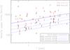 |
Fig. A.3
90% upper limits on velocity broadening obtained in the 0.8′ region versus RGS temperature (the red arrows provide the conservative limits measured with the best-fit spatial broadening, see Sect. 4.2). The sound speed and the fractions of thermal energy in turbulence are shown. |
| Open with DEXTER | |
|
Fig. A.4
Left panel: 90% conservative upper limits on Mach number versus temperature. Point size refers to the physical scale and the color is coded according to the central entropy, K0, in units of keV cm-2. The lines show the upper limits on Mach number averaged in the four ranges of physical scales to underline its dependence on the source distance. Right panel: same as before, but here the limits on Mach number are scaled by the 1/3rd power of the physical scale for a comparison between sources at different redshift (assuming Kolmogorov turbulence, see Sect. 5.2). |
|
| Open with DEXTER | |
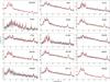 |
Fig. A.5
RGS spectral fits for the (−1.7′,+1.7′) region with the 7−25 Å spatial broadening profile (Part I). For displaying purposes, the spectra were combined using the XMM-SAS task rgscombine. |
| Open with DEXTER | |
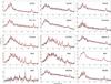 |
Fig. A.6
RGS spectral fits for the (−1.7′,+1.7′) region with the 7−25 Å spatial broadening profile (Part II). For displaying purposes, the spectra were combined using the XMM-SAS task rgscombine. |
| Open with DEXTER | |
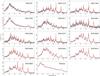 |
Fig. A.7
RGS spectral fits for the (−1.7′,+1.7′) region with the 7−25 Å spatial broadening profile (Part III). For displaying purposes, the spectra were combined using the XMM-SAS task rgscombine. |
| Open with DEXTER | |
Velocity broadening upper limits and total line widths.
Additional results and physical properties.
© ESO, 2015
Current usage metrics show cumulative count of Article Views (full-text article views including HTML views, PDF and ePub downloads, according to the available data) and Abstracts Views on Vision4Press platform.
Data correspond to usage on the plateform after 2015. The current usage metrics is available 48-96 hours after online publication and is updated daily on week days.
Initial download of the metrics may take a while.