| Issue |
A&A
Volume 575, March 2015
|
|
|---|---|---|
| Article Number | A9 | |
| Number of page(s) | 27 | |
| Section | Interstellar and circumstellar matter | |
| DOI | https://doi.org/10.1051/0004-6361/201425020 | |
| Published online | 11 February 2015 | |
Online material
Appendix A: LTE analysis of [CI]
|
Fig. A.1
Velocity channel maps at 1 km s-1 width of the optical depth τ1 → 0 of the [C I] 1 → 0 line, estimated assuming LTE conditions in M17 SW. |
|
| Open with DEXTER | |
Following Frerking et al. (1989) and Schneider et al. (2003, their Appendix A), the optical depths of the [C I] J = 1 → 0 and J = 2 → 1 lines can be estimated from the excitation temperature and the peak intensity of both lines, assuming a beam filling factor of unity. Knowing the excitation temperature and the optical depth of the J = 1 → 0 line, the column density N([C I]) can be computed as well. Figures A.1 and A.2 shows the channel maps corresponding to the optical depths of both [C I] lines, while Fig. A.3 shows the channel maps of the [C I] column density, as estimated assuming LTE conditions.
|
Fig. A.2
Velocity channel maps at 1 km s-1 width of the optical depth τ2 → 1 of the [C I] 2 → 1 line, estimated assuming LTE conditions in M17 SW. |
|
| Open with DEXTER | |
|
Fig. A.3
Velocity channel maps at 1 km s-1 width of the column density (cm-2) of [C I] (in log 10 scale), estimated using the excitation temperature from Fig. 6. |
|
| Open with DEXTER | |
Appendix B: Non-LTE excitation analysis of [C I]
Following the procedure described in (Pérez-Beaupuits et al. 2007, 2009), we use the radiative transfer code RADEX (van der Tak et al. 2007) to create a data cube containing the intensities, as well as the excitation temperatures and optical depths of the two [C I] transitions, in function of a range of kinetic temperatures TK, number densities n(H2) (i.e., excitation conditions), and column densities per line width N/ ΔV. The collision rates used were taken from the LAMDA database (Schöier et al. 2005).
We only used collisions with H2 since this is the most abundant molecule. Other collision partners can be H and He. Although their collision cross sections are comparable, H2 is about 5 times more abundant than He, and H is at least one order of magnitude less abundant than H2 in the dense cores of molecular clouds (e.g., Meijerink & Spaans 2005). Hence, including H and He as additional collision partners would not produce a significant change in our results. We also assumed a homogeneous spherical symmetry in the clumps for the escape-probability formalism.
The original RADEX code was modified to include dust background emission as a diluted blackbody radiation field, as in Poelman & Spaans (2005) and Pérez-Beaupuits et al. (2009). The total background radiation is modeled as a composite between the cosmic background radiation (CMB), assumed to be a blackbody function at 2.73 K, and the diluted dust radiation estimated as τdust × B(Tdust), where B(Tdust) is the Planck function and the dust continuum optical depth τdust(λ) is defined by Hollenbach et al. (1991) as τdust(λ) = τ100 μm(100 μm /λ). We adopted an average dust background temperature Tdust = 50 K and the high FIR opacity τ100 μm = 0.106 found by Meixner et al. (1992) in M17SW.
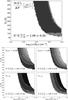 |
Fig. B.1
Excitation map (top panel) for the [C I] |
| Open with DEXTER | |
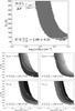 |
Fig. B.2
Excitation map (top panel) for the [C I] |
| Open with DEXTER | |
We assume that the emission collected by the beam has a homogeneous elliptical Gaussian distribution and that the coupling factor of our beam to the source distribution is unity, so we can compare directly with the output of RADEX, which is the Rayleigh-Jeans equivalent radiation temperature TR emitted by the source.
We explored all the possible excitation conditions within the given range that can lead to the observed radiation temperatures and the line ratios between the two [C I] lines. The line ratios and the peak temperature of the lower-J line involved in each ratio were used to constrain the excitation conditions. Including the rms of the observed spectra and uncertainties in all the assumptions mentioned above, a 20% error of the ratios and peak temperatures are used to define a range of values for TK, n(H2), and N/ ΔV within which the RADEX output is selected as a valid solution.
The volume density explored ranges between 102 cm-3 and 104 cm-3, the kinetic temperature varies from 10 K to 500 K, and the column density per line width lies between 1010cm-2 km-1 s and 1020cm-2 km-1 s. Since the optical depth, and the line intensities, are proportional to the column density per line width N/ ΔV, we generated the RADEX data cube assuming the ΔV = 1km s-1 of the velocity channels in the re-sampled spectra. In order to constrain the solutions, we fit the line ratio between the peak temperatures of the transitions and the radiation temperature of the lower transition (J = 1 → 0), which are R ~ 1.08 and TR ≈ Tmb = 31.9 K at offset position (−130′′,−10′′), and R ~ 1.06 and TR ≈ Tmb = 22.4 K at offset position (−130′′, −70′′).
Figures B.1 to B.2 show gray scale and contour maps of the excitation conditions found to reproduce the observed [C I] line ratios and peak temperatures at the offset positions (−130′′, −10′′) and (−130′′, −70′′), respectively. The values shown correspond to the average of all the possible N/ ΔV, Tex, and τ found for each pair of excitation conditions (n(H2) and TK). The curvature in the solutions depict the dichotomy between the kinetic temperature and the density of the collision partner. In other words, solutions for the observed values can be found for higher temperatures and lower densities, but also for lower TK and higher n(H2). The column density per line width does not change significantly along the solution curve, but it does change slightly across the curves, and especially at lower (< 100 K) kinetic temperatures. This means that for a given kinetic temperature, N/ ΔV will show a small variation in function of density.
|
Fig. C.1
Example of the scatter plots between the pixel values of the velocity-integrated intensity maps of two different line tracers, and the corresponding correlation coefficient obtained using Eq. (C.1.) |
|
| Open with DEXTER | |
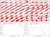 |
Fig. C.2
Example of the scatter plots between the pixel values (K km s-1) of the velocity channel maps of the 12CO J = 1 → 0 (X-axis) and J = 2 − 1 (Y-axis) transitions (top left), and the [C I] 370 μm (X-axis) and 13CO J = 2 → 1 (Y-axis) lines (top right). The corresponding correlation coefficient r at each velocity channel, is shown in the bottom panels. |
| Open with DEXTER | |
Appendix C: Correlation between line tracers
In order to verify the apparent spatial correlation between two species, we use the correlation between a specific pixel value of a map, and the same pixel in the map of another tracer. This can be done only in the maps with the same dimensions and spatial resolutions. Therefore, we first convolved all the maps to the larger beam size (24′′) of the C![]() O J = 1 − 0 line, and we used the SOFIA/GREAT map of the [C II] 158 μm line (which covers the smaller region) as a template to create all the [C I] and CO maps. The sample correlation coefficient commonly used to estimate rxy between the images X and Y is the Pearson’s product-moment correlation coefficient defined by (Pearson 1920; Rodgers & Nicewander 1988),
O J = 1 − 0 line, and we used the SOFIA/GREAT map of the [C II] 158 μm line (which covers the smaller region) as a template to create all the [C I] and CO maps. The sample correlation coefficient commonly used to estimate rxy between the images X and Y is the Pearson’s product-moment correlation coefficient defined by (Pearson 1920; Rodgers & Nicewander 1988), 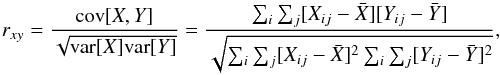 (C.1)where Xij and Yij are the pixel values of two given maps or images (e.g., [C II] and 12CO J = 1 → 0), and
 ![]() and
and ![]() are the average pixel value of the respective maps. We note that the uncertainty of the correlation coefficient can be approximated as
are the average pixel value of the respective maps. We note that the uncertainty of the correlation coefficient can be approximated as ![]() , and since we have maps with n = 31 × 18 = 558 pixels, the uncertainty will always be between 10-2 and 10-3. This correlation is applied to the velocity integrated intensity maps, and to the 1 km s-1 width channel maps. We note that because of the positive correlation between the intensities of different tracers, rxy ranges between 0 and 1. As proof of concept, the scatter plot and the associated correlation coefficient between the velocity-integrated intensity of several line tracers is shown in Fig. C.1. The application of the scatter plot to the channel maps is shown in Fig. C.2 for two test cases. We note that the correlation between the velocity-integrated intensity, as well as the channel maps, of the J = 1 → 0 and J = 2 → 1 transitions of 12CO is very good, even at the faintest emission of the lower velocity (> 3.5 km s-1) channels, but the good correlation is lost at the higher velocity (> 28.5 km s-1) channels. In the case of the [C I] 370 μm (X-axis) versus 13CO J = 2 → 1 (Y-axis), the pixel values are more scattered at the lower (< 16km s-1) and higher (> 22km s-1) velocity channels because the line intensities are fainter and, hence, those channel maps are more affected by noise.
, and since we have maps with n = 31 × 18 = 558 pixels, the uncertainty will always be between 10-2 and 10-3. This correlation is applied to the velocity integrated intensity maps, and to the 1 km s-1 width channel maps. We note that because of the positive correlation between the intensities of different tracers, rxy ranges between 0 and 1. As proof of concept, the scatter plot and the associated correlation coefficient between the velocity-integrated intensity of several line tracers is shown in Fig. C.1. The application of the scatter plot to the channel maps is shown in Fig. C.2 for two test cases. We note that the correlation between the velocity-integrated intensity, as well as the channel maps, of the J = 1 → 0 and J = 2 → 1 transitions of 12CO is very good, even at the faintest emission of the lower velocity (> 3.5 km s-1) channels, but the good correlation is lost at the higher velocity (> 28.5 km s-1) channels. In the case of the [C I] 370 μm (X-axis) versus 13CO J = 2 → 1 (Y-axis), the pixel values are more scattered at the lower (< 16km s-1) and higher (> 22km s-1) velocity channels because the line intensities are fainter and, hence, those channel maps are more affected by noise.
 |
Fig. D.1
Example of the steps in the method to estimate the spatial association between two emission lines. The top panels shows the channel maps of the 1 km s-1 integrated intensity (in K km s-1 ) of the [C II] 158 μm (left) and [C I] 609 μm (right) lines. The contour lines correspond to the threshold of 10% of their global peak intensities (136.4 K km s-1 and 54.6 K km s-1 for [C II] and [C I], respectively). The middle panels are the binary images obtained after applying the intensity threshold to the original channel maps. The bottom panel shows the result of multiplying the two binary images, which corresponds to the region where the emission of both [C II] and [C I] lines are associated in a particular velocity channel (in this case 15.5–16.5 km s-1). |
| Open with DEXTER | |
|
Fig. D.2
Histograms of the fraction of the region mapped where two line tracers are associated at each 1 km s-1 width velocity channel. The corresponding correlation coefficient Rxy obtained using Eq. (C.1) for each channel map is shown with a continuous line. |
|
| Open with DEXTER | |
Appendix D: Spatial association in channel maps
We use a simple method to estimate the fraction of the region mapped where two emission lines are associated in narrow (1 km s-1) width channel maps. All maps are first convolved to the lowest spatial resolution (24′′ FWHM beam) of the C![]() O J = 1 → 0 map in order to increase the S/N, and the size of the [C I], 12CO and isotope maps is limited to the region mapped in [C II] by using the [C II] data cube as a template in GILDAS/CLASS. In this way, we produce spectral cubes with the same dimensions and number of pixels.
O J = 1 → 0 map in order to increase the S/N, and the size of the [C I], 12CO and isotope maps is limited to the region mapped in [C II] by using the [C II] data cube as a template in GILDAS/CLASS. In this way, we produce spectral cubes with the same dimensions and number of pixels.
Then we determine which region of the maps have significant emission. This can be done naturally by using the rms (noise) level of the spectra corresponding to each pixel in the map (i.e., a 3σ level detection), or by defining a threshold for the intensities. Since our maps (especially that of the [C II] line) are not homogeneously sampled, the rms level varies among the different pixels. Hence, we prefer to use a fraction of the global peak (maximum) integrated intensity found among all the channel maps as a threshold. This provides a unique value that is used to determine whether the emission of some region (pixel) in a particular channel map is significant or not.
We create binary images for each channel map by assigning a zero to all the pixels with intensity values lower than the threshold, and a value of unity to all the pixels that have intensity values larger than or equal to the threshold. We use a conservative value of 10% of the global peak emission for the threshold, which is about ten times higher than the noise level in most of the channel maps of all the lines we consider. This conservative value is used in order to avoid the association of emission levels in one image that would be considered noise in another image.
Then we multiply each binary channel map image of the two line tracers we want to compare, to see if there are regions where the two emissions are associated in that particular velocity channel. The product image would contain pixels with 1’s in regions where both line tracers have significant emission, and 0’s otherwise. Thus, adding up all the pixels from the product image, and dividing by the total number of pixels, we obtain the fraction of the region mapped where the emission from both lines is associated. An example of this procedure, applied to the [C II] 158 μm and [C I] 609 μm lines, is shown in Fig. D.1.
With this method we can estimate the fraction, and where in the region mapped, two line tracers are associated at each velocity channel. The fraction of the region mapped can be compared with the correlation coefficient described in Appendix C. Test cases of this are shown in Fig. D.2.
Appendix E: [C II] emission associated with the three gas phases
Subtracting the scaled up spectra of [C I] 609 μm, 12CO J = 1 → 0, and the velocity-resolved optical depth τ(H I) from the [C II] spectra, we obtained a residual [C II] emission that
should be mostly associated with the ionized hydrogen gas (H II). When subtracting the maximum (channel by channel) between the tracers of the H2 gas (e.g., [C I] 609 μm and 12CO J = 1 → 0, or [C I] 609 μm and C![]() O J = 2 → 1) from the original [C II] spectra, we obtain a second residual [C II] emission that is expected to be mostly associated with the neutral (H I) and ionized atomic gas (H II). The difference between these residual spectra and the original [C II] spectra gives the [C II] emission that is mostly associated with the H2 gas. Subtracting the [C II] emission that is mostly associated with the H2 gas and the first residual spectra associated with H II from the original [C II] spectra would lead to a third residual [C II] emission that is mostly associated with the neutral atomic hydrogen gas, H I. The corresponding column densities can be estimated assuming the LTE conditions and Eq. (2). The velocity channel maps of the residual [C II] emission associated to each of the gas phases, as estimated with model (2) from Table 1, is shown in Fig. E.1.
O J = 2 → 1) from the original [C II] spectra, we obtain a second residual [C II] emission that is expected to be mostly associated with the neutral (H I) and ionized atomic gas (H II). The difference between these residual spectra and the original [C II] spectra gives the [C II] emission that is mostly associated with the H2 gas. Subtracting the [C II] emission that is mostly associated with the H2 gas and the first residual spectra associated with H II from the original [C II] spectra would lead to a third residual [C II] emission that is mostly associated with the neutral atomic hydrogen gas, H I. The corresponding column densities can be estimated assuming the LTE conditions and Eq. (2). The velocity channel maps of the residual [C II] emission associated to each of the gas phases, as estimated with model (2) from Table 1, is shown in Fig. E.1.
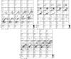 |
Fig. E.1
Velocity channel maps at 1 km s-1 width of the [C II] emission (in K km s-1 ), associated with the H II (top left), H I (top right), and H2 (bottom) gas phase, as estimated with model (2) from Table 1. Contours are 20%, 40%, 60%, 80%, and 100% of the respective peak emissions |
| Open with DEXTER | |
© ESO, 2015
Current usage metrics show cumulative count of Article Views (full-text article views including HTML views, PDF and ePub downloads, according to the available data) and Abstracts Views on Vision4Press platform.
Data correspond to usage on the plateform after 2015. The current usage metrics is available 48-96 hours after online publication and is updated daily on week days.
Initial download of the metrics may take a while.