| Issue |
A&A
Volume 575, March 2015
|
|
|---|---|---|
| Article Number | A79 | |
| Number of page(s) | 17 | |
| Section | Interstellar and circumstellar matter | |
| DOI | https://doi.org/10.1051/0004-6361/201423569 | |
| Published online | 26 February 2015 | |
Online material
Appendix A: Effects of binning and cropping on the PDF
Figure A.1 shows the effect on the PDF of varying the binsize. We started first from the original column density map on a 14′′ grid, which approximately corresponds to Nyquist sampling for an angular resolution of the data of 36′′. It becomes obvious that there is basically no effect on the derived values of Av (peak), Av (DP), and slope. For the fit, we fixed only the width of the PDF in order to avoid the lower column density peak, arising from a seperate component, being taken into account. A binsize of 0.1 turns out to be the best choice for our data because finer sampling (0.05) increases the statistical noise for the higher column density range, and a lower sampling (0.2) smoothes out features in the PDF that can still be significant.
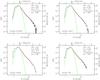 |
Fig. A.1
PDFs obtained from the orginal (not LOS-corrected) Auriga column density map with different bin sizes (0.05, 0.1, and 0.2) and a PDF with a binsize of 0.1 but on a grid of 36′′ (lower, right panel). The vertical dashed line indicates the noise level of the map. The left y-axis gives the normalized probability p(η), the right y-axis the number of pixels per log bin. The upper x-axis is the visual extinction and the lower x-axis the logarithm of the normalized column density. The green curve indicates the fitted PDF (we fixed the width of the PDF in order to avoid the low column density component being included). The red line indicates a power-law (linear regression) fit to the high Av tail (the start- and end-point were fixed to the same values for each PDF). Inside each panel, we give the value where the PDF peaks (Apk), the deviation point from lognormal to power-law tail (DP), the dispersion of the fitted PDF (ση), the slope s and the X2 of the fit, and the exponent α of an equivalent spherical density distribution. |
| Open with DEXTER | |
In Fig. A.2 we investigate the effect of “field-cropping”, which is how the PDF shape changes when only pixels above a certain threshold are considered, using the Auriga cloud as an example. First, we observe that for high column density ranges, i.e. above the peak of the lognormal distribution, the PDF is only represented by a power-law tail all with the same slope, independent of Av-threshold. Small variations in the PDF shape are due to the normalization process. (The average column density changes for each threshold-value). As a consequence, PDFs obtained by “cropping” images at high column densities, such as PDFs for IRDCs in IR-quiet molecular clouds, should thus be strongly dominated by the power-law tail. This was recently confirmed observationally by Schneider et al. (2014). Toward the low column density range, we constructed PDFs above threshold values of Av = 0.2 (noise level), Av = 0.5, and Av = 0.8 (background level). We do not observe a significant effect on the PDF shape when we change the threshold, though it is clear that for the lowest column densities, the clouds in our Herschel maps are not completely sampled.
|
Fig. A.2
Left: column density map of Auriga (without correction for LOS-contamination), showing the emission distribution at various thresholds of Av. The colors correspond to the PDFs (right panel) constructed above Av levels of 0.8, 2, 4, 6, and 8. The y-axis gives the normalized probability p(η), and the x-axis the visual extinction. |
|
| Open with DEXTER | |
|
Fig. B.1
Left: Herschel column density map of the Auriga cloud in [cm-2]. The black dashed polygon indicates the pixels from which the PDF was determined. This is the common overlap region of SPIRE and PACS in which the column density map was determined from the SED fit using the 4 wavelengths. Outside this polygon, the fit relies only on SPIRE and it less reliable. The white polygon outlines the area used for determining the background/foreground level of contamination of the map. Right: SPIRE 250 μm map in units [MJy/sr]. |
|
| Open with DEXTER | |
Appendix B.2: Herschel maps of molecular clouds
All maps presented in this paper – and in the furthcoming ones – were treated in the same way with regard to data reduction and determination of the column density maps. For the data reduction of the Herschel wavelengths, we used the HIPE10 pipeline, including the destriper task for SPIRE (250, 350, 500 μm), and HIPE10 and scanamorphos v12 (Roussel et al. 2013) for PACS (70′′ and 160′′, Poglitsch et al. 2010). The SPIRE (Griffin et al. 2010) maps include the turnaround-data (when the satellite changed mapping direction for the scan) and were calibrated for extended emission.
The procedure for making column density and temperature maps is independent of the data reduction process and follows the scheme described in Schneider et al. (2012). The column density maps were determined from a pixel-to-pixel graybody fit to the red wavelength of PACS (160 μm) and SPIRE (250, 350, 500 μm). We did not include the 70 μm data because we focus on the cold dust and not UV-heated warm dust (see Sect. 4.1 in Russeil et al. 2013 for more details on this issue). The maps were first convolved to have the same angular resolution of 36′′ and then regridded on a 14′′ raster. All maps have an absolute flux calibration, using the zeropointcorrection task in HIPE10 for SPIRE and IRAS maps for PACS.
|
Fig. B.2
Left: Herschel column density map of the Maddalena cloud in [cm-2]. All other parameters as in Fig. B.1. Right: SPIRE 250 μm map in units [MJy/sr]. |
|
| Open with DEXTER | |
|
Fig. B.3
Left: Herschel column density map of NGC 3603 in [cm-2]. The contour levels are 3, 6, 10, and 20 × 1021 cm-2. All other parameters as in Fig. B.1. Right: SPIRE 250 μm map in units [MJy/sr]. The gray star indicates the location of the central cluster. |
|
| Open with DEXTER | |
|
Fig. B.4
Left: Herschel column density map of Carina in [cm-2]. The contour levels are 5, 10, and 20 × 1021 cm-2. All other parameters as in Fig. B.1. Right: SPIRE 250 μm map in units [MJy/sr]. The gray stars indicate the location of the OB clusters Tr14 and Tr16. |
|
| Open with DEXTER | |
The correction for SPIRE works in such a way that that a cross-calibration with Planck maps at 500 and 350 μm is performed. We emphasize that such a correction is indispensable for accurately determining column density maps. For the SED fit, we fixed the specific dust opacity per unit mass (dust+gas) approximated by the power law κν = 0.1 (ν/ 1000 GHz)β cm2/g and β = 2 and left the dust temperature and column density as free parameters. We checked the SED fit of each pixel and determined from the fitted surface density the H2 column density. For the transformation H2 column density into visual extinction, we used the conversion formula N(H2) /Av = 0.94 × 1021 cm-2 mag-1 (Bohlin et al. 1978). The angular resolution of the column density maps is ~36′′, and they are shown in Figs. B.1 to B.4, together with SPIRE 250 μm images. We estimate the final uncertainties in the Herschel column density maps to be around ~30–40%, mainly arising from the uncertainty in the assumed form of the opacity law, and possible temperature gradients along the LOS (see Roy et al. 2014, for details on the dust opacity law and Russeil et al. 2013, for a quantitative discussion on the various error sources).
© ESO, 2015
Current usage metrics show cumulative count of Article Views (full-text article views including HTML views, PDF and ePub downloads, according to the available data) and Abstracts Views on Vision4Press platform.
Data correspond to usage on the plateform after 2015. The current usage metrics is available 48-96 hours after online publication and is updated daily on week days.
Initial download of the metrics may take a while.