| Issue |
A&A
Volume 574, February 2015
|
|
|---|---|---|
| Article Number | A136 | |
| Number of page(s) | 20 | |
| Section | Astrophysical processes | |
| DOI | https://doi.org/10.1051/0004-6361/201424451 | |
| Published online | 10 February 2015 | |
Online material
Appendix A: Most probable in general case
The MP2 estimators, ![]() and
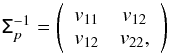
and ![]() , have to satisfy Eqs. (8) and (9) simultaneously. These relations can be solved using the fully developed expression of f2D, including the terms of the inverse matrix
, have to satisfy Eqs. (8) and (9) simultaneously. These relations can be solved using the fully developed expression of f2D, including the terms of the inverse matrix ![]() :
:  (A.1)leading to
 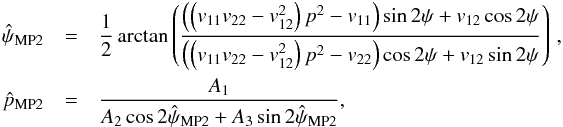 (A.2)with
 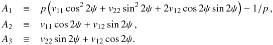 (A.3)This analytical solution only depends on the input measurements (p, ψ) and the covariance matrix Σp. Because the polarization fraction must be positive, there is a lower limit of the S/N so that
 ![]() . In that case,
. In that case, ![]() is not constrained anymore and can be chosen to be any possible value. We set it equal to
is not constrained anymore and can be chosen to be any possible value. We set it equal to
the measurement ψ. Moreover, this expression can be simplified when ρ = 0, which implies that v12 = 0, leading to 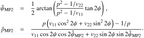 (A.4)In the canonical case (v12 = 0,
 ![]() ), we recover the expression derived by Quinn (2012):
), we recover the expression derived by Quinn (2012): 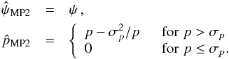 (A.5)
(A.5)
Appendix B: Bayesian posterior PDF
We illustrate the shape of the posterior PDF in Fig. B.1, where B2D(p0,ψ0 | p,ψ,Σp) is shown at four levels of the S/N and five couples of (ε, ρ). It is interesting to notice that the posterior PDF allows the polarization fraction to be zero at low S/N, when these values were rejected by the PDF (see Appendix B of PMA I). Moreover, the posterior PDF peaks at the location of the measurements used to compute it. As largely emphasized in PMA I, we also recall that once the effective ellipticity of the covariance matrix departs from the canonical simplification, the PDFs are sensitive to the initial true polarization angle ψ0.
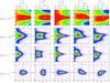 |
Fig. B.1
Posterior probability density functions B2D(p0,ψ0 | p,ψ,Σp) computed for the most probable measurements (p, ψ) of the f2D distribution (crosses), which were obtained for a given set of true polarization parameters ψ0 = 0° and p0 = 0.10 (dashed lines) and various configurations of the covariance matrix, at four levels of S/N p0/σp,G = 0.1,0.5,1, and 5 (top to bottom). The scales of the p0 and ψ0 axes may vary from one row to the next in order to focus on the interesting part of the PDF. The black contours provide the 90, 70, 50, 20, 10, 5, 1, and 0.1% levels. |
| Open with DEXTER | |
Appendix C: Mean Bayesian posterior analytical expression
In the canonical case, the MB estimator of the polarization fraction p takes a simple analytical expression. The Bayesian posterior on p is given in this case by 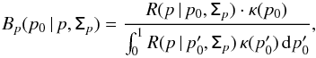 (C.1)where κ is the prior chosen equal to one over the definition range ([0,1]), and R denotes the Rice (1945) function which is defined by
 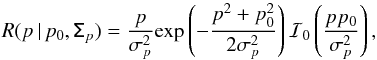 (C.2)where ℐ0(x) is the zeroth-order modified Bessel function of the first kind (Gradshteyn & Ryzhik 2007), and σp = σQ/I0 = σU/I0 is the characteristic noise level of the polarization fraction.
The MB estimator and the posterior variance take the following forms 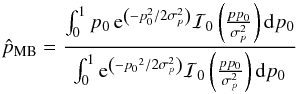 (C.3)and
 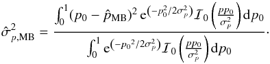 (C.4)If we assume in a first approximation that the integral of p0 over [ 0,1 ] can be taken over [ 0, + ∞) (which is fine at high S/N), and we use the formula of Prudnikov et al. (1986),
 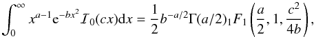 (C.5)where Γ is the Gamma function,
 ![]() the confluent hypergeometric function of the first kind, and a, b, and c all positive reals, we can derive
the confluent hypergeometric function of the first kind, and a, b, and c all positive reals, we can derive 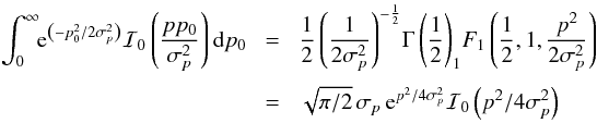 (C.6)\pagebreak
and 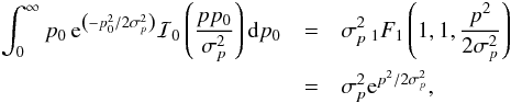 (C.7)and finally
 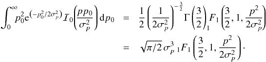 (C.8)We finally obtain the simple expression of the MB estimator and the associated Bayesian variance:
 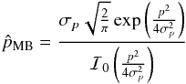 (C.9)and
 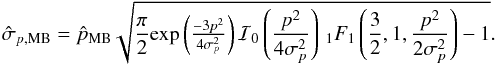 (C.10)As shown in Fig. C.1, this analytical approximation gives less than 0.15% of relative error at low S/N compared to the exact
 ![]() estimate and less than 0.05% for the associated uncertainty. This small departure quickly tends to 0 for a S/N> 4. Thus these expressions may be used to speed up the computing time when the canonical simplification may be assumed.
estimate and less than 0.05% for the associated uncertainty. This small departure quickly tends to 0 for a S/N> 4. Thus these expressions may be used to speed up the computing time when the canonical simplification may be assumed.
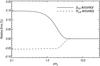 |
Fig. C.1
Accuracy of the approximate analytical expression of the Bayesian estimates of the polarization fraction |
| Open with DEXTER | |
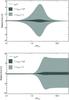 |
Fig. C.2
Accuracy of the generalized approximate analytical expression of the Bayesian estimates |
| Open with DEXTER | |
We explore in Fig. C.2 to the extent at which the canonical simplification may be done in the presence of an effective ellipticity of the covariance matrix. In this more general case, we suggest changing σp into σp,G in the Eqs. (C.9) and (C.10). The relative error between the approximate estimate and the exact Bayesian estimate has been explored in two regimes of the covariance matrix, the low (1 <εeff< 1.1) and tiny (1 <εeff< 1.01) regimes. Three domains are observed in the top panel of Fig. C.2 dealing with the accuracy of the ![]() estimate: i) at low S/N (<1), the bias on p is so large that the presence of an effective ellipticity does not significantly affect the estimate in comparison; ii) for an intermediate range of the S/N (1 <S/N< 4), the effective ellipticity of the Σp significantly affects the Bayesian estimate so that the departure of the analytical approximation from the exact estimate becomes important; iii) at high S/N (>4), the noise is so low that the Bayesian estimate is not sensitive to the asymmetry of the covariance matrix anymore. Consequently, the approximate analytical expression provides very good estimates of
estimate: i) at low S/N (<1), the bias on p is so large that the presence of an effective ellipticity does not significantly affect the estimate in comparison; ii) for an intermediate range of the S/N (1 <S/N< 4), the effective ellipticity of the Σp significantly affects the Bayesian estimate so that the departure of the analytical approximation from the exact estimate becomes important; iii) at high S/N (>4), the noise is so low that the Bayesian estimate is not sensitive to the asymmetry of the covariance matrix anymore. Consequently, the approximate analytical expression provides very good estimates of ![]() for S/N< 1 and S/N> 4, and 5% to 0.5% of relative error for intermediate 1 <S/N< 4 in the low and tiny regimes of the covariance matrix, respectively. In the extreme regime of the covariance matrix, the relative error increases up to 20%.
for S/N< 1 and S/N> 4, and 5% to 0.5% of relative error for intermediate 1 <S/N< 4 in the low and tiny regimes of the covariance matrix, respectively. In the extreme regime of the covariance matrix, the relative error increases up to 20%.
Concerning the accuracy of the Bayesian approximate estimate ![]() of the polarization fraction uncertainty (bottom panel), the agreement is better than 0.1% for S/N< 1, and about 8% S/N> 1 in the low regime, and 1% in the tiny regime. Because the uncertainty becomes small compared to the polarization fraction at high S/N, up to 8% of error in
of the polarization fraction uncertainty (bottom panel), the agreement is better than 0.1% for S/N< 1, and about 8% S/N> 1 in the low regime, and 1% in the tiny regime. Because the uncertainty becomes small compared to the polarization fraction at high S/N, up to 8% of error in ![]() is still acceptable for this approximation.
is still acceptable for this approximation.
© ESO, 2015
Current usage metrics show cumulative count of Article Views (full-text article views including HTML views, PDF and ePub downloads, according to the available data) and Abstracts Views on Vision4Press platform.
Data correspond to usage on the plateform after 2015. The current usage metrics is available 48-96 hours after online publication and is updated daily on week days.
Initial download of the metrics may take a while.