| Issue |
A&A
Volume 572, December 2014
|
|
|---|---|---|
| Article Number | A8 | |
| Number of page(s) | 8 | |
| Section | Cosmology (including clusters of galaxies) | |
| DOI | https://doi.org/10.1051/0004-6361/201424418 | |
| Published online | 19 November 2014 | |
Online material
Appendix A: Kernel density estimation
In the simplest case, the probability density can be estimated as the binned density histogram. However, this estimate depends both on the bin widths and the location of the bin edges. A better way is to use kernel smoothing (e.g. Silverman 1986; Wand & Jones 1995; Feigelson & Jogesh Babu 2012), where the density is represented by a sum of kernels centred at the data points:  (A.1)The kernels K(x) are distributions (K(x) > 0, ∫K(x)dx = 1) of zero mean and of a typical width h. The width h is an analogue of the bin width, but there are no bin edges to worry about.
To create our density estimation we use the popular B3 spline function  (A.2)This kernel is well suited for estimating densities – it is compact, differing from zero only in the interval x ∈ [−2,2], and it conserves mass: ∑ iB3(x − i) = 1 for any x.
In many papers (e.g. Vio et al. 1994; Fadda et al. 1998; Ferdosi et al. 2011) it has been shown that kernel smoothing is the best and recommended choice for density estimation. It is more robust and reliable than other simpler methods and provides comparable (or better) results than methods with high computational costs (e.g. the maximum likelihood technique).
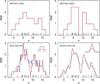 |
Fig. A.1
Upper row: probability density estimation using binning. In the left and right panels, the bin width is the same but the centre of the bin is shifted. Bottom row: density estimation using kernel smoothing. In the bottom left panel the simplest box kernel is used, in the bottom right panel the B3 spline kernel is used. The kernel shape and size is shown in the upper-right corner of the figures. The rug plot on the bottom axis shows the data points that were used for density estimation. |
| Open with DEXTER | |
To illustrate the use of kernel smoothing, in Fig. A.1 we show the estimated probability density function using either binning the data or kernel smoothing with two types of kernels (the box and B3 spline kernels). The upper row in Fig. A.1 demonstrates density estimation using binning, where the bin widths are the same but the bin centres are slightly shifted. We see that the resulting density estimate may depend strongly on the chosen bin locations.
The lower-left panel in Fig. A.1 demonstrates density estimation using the simplest box kernel. The kernel width is the same as box width for binned density estimates above. Even the simplest box kernel reveals the details in density distribution; however, the resulting distribution function is not smooth. To get a smooth density distribution, a smooth kernel should be used. The kernel density estimates using B3 spline kernels are shown in the lower-right panel of Fig. A.1. To show that the results of kernel smoothing are quite robust, we doubled the kernel width and compared the probability density estimates as shown in Fig. A.1.
Appendix B: Examples of the Rayleigh (Z-squared) statistic
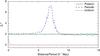 |
Fig. B.1
Z-squared statistics for three cases. The green line shows the Z-squared statistic for a Poisson sample. The blue line shows the statistic for a periodic signal, where the period for each datapoint is drawn from a Gaussian distribution centred at 7 h-1 Mpc with a standard deviation of 0.5 h-1 Mpc. The red line shows the statistic for data points with an uniform point distribution – see text for more information. |
| Open with DEXTER | |
To illustrate how the Z-squared statistic works, we generated three datasets and calculated the Rayleigh statistics for them. The results are shown in Fig. B.1. In the first case, we generated a Poisson distribution (green line). For a Poisson sample, the statistic gives an average value of 2. In the second case, we added some periodicity to the sample (blue line). We generated point distributions with the same (zero) phase and with periods chosen from a Gaussian distribution centred at 7 h-1 Mpc with a standard deviation of 0.5 h-1 Mpc, and added these together. In Fig. B.1 we see that the Z-squared statistic recovers the period well. In the third case, we generated a uniform distribution of points (red line). For that, we divided the test filament into N (the number of points) equal regions and in each region we put one point, selected from a uniform distribution. This ensures that we get points that are more homogeneously distributed along the filament and the Z-squared statistic gives the value zero. We can conclude that if the value of the statistic lies above 2, there is some periodicity in the data. Conversely, if it is below 2, it describes a more homogeneous distribution. Additionally, the peaks in the Z-squared statistic show that there is preferred periodicity in the data with the scale of the peak position.
It is known that for the uniform distribution of points, the Z-squared statistic is distributed as the chi-square with two degrees of freedom (see e.g. Wall & Jenkins 2012). So its expected value is 2, as seen in Fig. B.1.
© ESO, 2014
Current usage metrics show cumulative count of Article Views (full-text article views including HTML views, PDF and ePub downloads, according to the available data) and Abstracts Views on Vision4Press platform.
Data correspond to usage on the plateform after 2015. The current usage metrics is available 48-96 hours after online publication and is updated daily on week days.
Initial download of the metrics may take a while.