| Issue |
A&A
Volume 572, December 2014
|
|
|---|---|---|
| Article Number | A66 | |
| Number of page(s) | 17 | |
| Section | Extragalactic astronomy | |
| DOI | https://doi.org/10.1051/0004-6361/201423555 | |
| Published online | 28 November 2014 | |
Online material
Appendix A: The line fitting procedure and narrow line subtraction
One of the problems in the measurements of the broad line parameters is the uncertainty in the narrow line subtraction, especially in the red peak of Hα and Hβ, since the narrow lines are right on top of the red peak in both broad lines. Therefore, to find uncertainties in the narrow line subtraction we performed several tests. Additionally, we considered the B-band absorption observed near the [SII] doublet in the Hα wavelength range.
Appendix A.1: Correction of the B-band absorption near [SII]
The B-band absorption is present in the red wing of the Hα line, near the narrow [SII] doublet (see Fig. A.1). To correct this absorption we used the template spectrum of NGC 4339, which was observed at the same night as Arp 102B with 2.1 m GHO telescope with resolution ~8–9 Å on Mar 26, 2003. Then we corrected the B-band absorption near the [SII] lines in the Hα spectral region.
In Fig. A.1, we illustrate the correction of the B-band absorption. As one can see in Fig. A.1 the absorption is well corrected, but in some spectra the residuals are still present. However, the residuals are weak and cannot affect the narrow line estimates, or the estimates of the red-peak position in Hα (see following section and Figs. A.2). Therefore, we accepted the parameters from the fits where the B-band absorption was not corrected.
Appendix A.2: Estimation of the narrow line emission
As we mentioned above, the uncertainties in the estimations of the broad line parameters come mainly from the subtraction of the narrow lines in the Hβ and Hα spectral range. It is hard to handle the removal of the narrow emission lines in Arp 102B, because the narrow lines are right on top of the red peak in the Hα and Hβ broad lines. We used two approaches to explore the uncertainty in the narrow line subtractions: i) fitting the narrow lines with Gaussian functions before and after the B-band absorption was corrected (as described in Sect. 2.2); and ii) estimation of the broad profile using spline fitting (using DIPSO). In Figs. A.2 and A.3, we illustrated the subtraction of the narrow lines using these two methods. In Fig. A.2 (fourth panel), we compared the broad Hα line profile obtained after the subtraction of the narrow lines using these two procedures (note that we fitted the spectra before and after the correction for the B-band absorption). As shown in Fig. A.3 (bottom panel), the fitted position of the blue and red peaks is also practically the same for Hβ for both procedures, therefore we used the Gaussian decomposition in our estimates of the narrow line contribution.
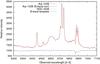 |
Fig. A.1
Correction of the Hα line on B-band absorption. The spectrum of NGC 4399 (shown below) is observed in the same epoch (Mar 26, 2003) as the spectra of Arp 102B. |
| Open with DEXTER | |
Appendix A.3: Correction of the fits using the ratio of the narrow lines
As we mentioned above, some parameters of the narrow lines are fixed in the spectral fit: first of all, the Gaussian velocity dispersions and shift for all narrow lines in the line wavelength range, as well as the ratio of the [OIII]4959,5007, which is fixed to 1:3 (Dimitrijević et al. 2007). Also, one cannot expect that the ratio of narrow lines changes over the period of several years. Therefore, one very clear way to test the robustness of the narrow line fittings is to compute the emission line ratios for each combined fit.
The timescale of the observations is long enough that there could be some variation in the narrow emission line ratios, but certainly over timescales of ~5–10 years there should not be major changes in the narrow line ratios (except of the random scatter). We calculated the narrow line ratios of [NII]/Hα, [OI]6300/Hα, [SII]6715/Hα, and [OIII]5007/Hβ. The line ratios in the Hα and Hβ wavelength range are presented in Fig. A.4, where dashed lines represent the averaged ratio and shaded regions the ±10% of the averaged value. As shown in the upper panels of Fig. A.4, there is not any trend in the line ratio variability during the monitored period. Consequently, we corrected those fits for which the narrow line ratios were significantly different from the mean value, i.e., the spectra with a big narrow line ratio difference have been refitted taking the constraint in the fit that the line ratio has to be in the frame of ±15% of the corresponding mean value. In the bottom panels of Fig. A.4, the line ratios are shown after the correction of a number of spectra.
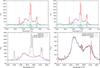 |
Fig. A.2
Multi-Gaussian fitting of the Hα wavelength range of the spectrum observed on Apr 02, 2003. Upper left: fitting of the spectra where the B-band absorption is not corrected. Upper right: the same except for the B-band corrected observed spectrum. In these two plots, the same Gaussians parameters (apart for the [SII] lines in which intensities are only increased) have been used. Bottom left: narrow lines removed using the DIPSO spline fitting of the broad component, compared with the 3-Gaussian broad-component fitting. Bottom right: comparison of the Hα broad component (after narrow lines subtraction) before and after the B-band absorption correction and the broad component obtained using the DIPSO spline fitting. The blue-peak position is the same, a slight difference is seen in the red peak. |
| Open with DEXTER | |
Appendix A.4: The broad line fit and estimates of parameter uncertainties
To find the broad line parameters of Hα and Hβ broad lines, we performed a Gaussian analysis, fitting the month-averaged broad line profiles. The broad profile was fitted with three Gaussian functions, corresponding to the blue, central, and red component (Fig. 5). Each Gaussian was described with three free parameters, i.e., in the fit procedure we have nine free parameters: three intensities, widths and shifts of Gaussian functions that describe the blue, central, and red part of the broad line.
Inspection of the obtained parameters from the fit, as well as several additional tests (changing slightly parameters), showed that the central component is often shifted to the blue (especially in Hα) and that, in some cases, this component has a big (unexpected) change in the shift. Additionally, we found that the position of the central component can significantly affect parameters of the peaks, especially the red peak. Therefore, we repeated the fitting procedure with three broad Gaussian functions, but putting the limits on the shift of the central component to be between –1000 km s-1 and 600 km s-1. Using this procedure we obtained an additional set of broad line parameters (parameters of the blue, central, and red Gaussians). Inspection of differences between the parameters obtained from the fits with and without constraint of the central component shift showed that the peak positions are not significantly changed, but the intensities of the red peak, the shift of the central component, and the widths of the components have been significantly changed.
We compared the error-bars from the fits with differences between the parameters from these two fitting procedures, and found that the error-bars of parameters are often significantly smaller than the differences between the parameters from both fits. Therefore, we calculated the averaged parameters
from the two fits, and accepted uncertainties (error-bars) as the discrepancy between the parameters from the two fits. The averaged broad line parameters and corresponding estimated uncertainties are given in Tables 2 (for Hα) and 3 (for Hβ).
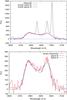 |
Fig. A.3
Upper panel: narrow lines removed in Hβ using the DIPSO spline fitting of the broad component, compared with the 3-Gaussian broad-component fitting. Bottom panel: comparison of the Hβ broad component (after narrow lines subtraction) using the 3-Gaussian and DIPSO spline fitting. The blue peak position is the same, a slight difference is seen in the red peak. |
| Open with DEXTER | |
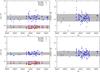 |
Fig. A.4
Ratio of the narrow emission line (labeled on plots) fluxes in the Hα (left panels) and Hβ (right panels) wavelength range during the monitored period. The narrow lines fluxes are calculated from the Gaussian fitting parameters as a sum of two components (one narrower fitting the line core and one broader fitting the line wings, see Sect. 2.2) The dashed lines with the shaded regions represent the mean value and the deviation of 10% from this. In upper panels, we obtained the ratios from the fit without any constraint, while in the bottom panels, the points with large scattering (from upper panels) have been corrected. |
| Open with DEXTER | |
© ESO, 2014
Current usage metrics show cumulative count of Article Views (full-text article views including HTML views, PDF and ePub downloads, according to the available data) and Abstracts Views on Vision4Press platform.
Data correspond to usage on the plateform after 2015. The current usage metrics is available 48-96 hours after online publication and is updated daily on week days.
Initial download of the metrics may take a while.