| Issue |
A&A
Volume 571, November 2014
|
|
|---|---|---|
| Article Number | L2 | |
| Number of page(s) | 5 | |
| Section | Letters | |
| DOI | https://doi.org/10.1051/0004-6361/201424796 | |
| Published online | 06 November 2014 | |
Online material
Appendix A: Testing the correlation significance
The significance of correlations in the DCF analysis was determined using simulations. To do so, we first estimated the PSD (power spectral density) slope of the γ-ray light curve following Vaughan (2005). The estimated PSD slope for 0716+714 is −(0.93±0.24). The next step is to generate the simulated light curves using the PSD slope. One can use the online available IDL code5. However, the simulated light curves using this code follow a Gaussian distribution, which is normally not the case for the observed light curves because a majority of them are burst-like events. This has to be taken into account while estimating the correlation significances (see Emmanoulopoulos et al. 2013, for details). We therefore checked the distribution of the observed γ-ray light curve and found that the underlying distribution is similar to a Gaussian one. We generated a series of 100 000 light curves using the online available IDL code. The next step is to sample the simulated light curves at the same times and bin widths as the observations. We cross-correlated the simulated γ-ray light curves with the observed PA curve. Finally, we calculated the distribution of the DCF values as a function of time lag. For each time delay, we estimated the 0.025 and 0.975 quantiles corresponding to the upper and lower limits of the 95% confidence bands. However, these confidence levels are obtained for a single trial; i.e. if we already know the time lag between the two light curves. Since we do not have the time lag information a priori, we always use a search window depending on the duration of observations. To correct for this effect (called the “look elsewhere effect”), one has to include the total number of trials, which is the number of data points in the given search window (for details see Sect. 4.1 in Vaughan 2005). For N points, the confidence level, ϵ, is (1 − (1 − ϵ) /N) × 100%; i.e. the 95% confidence level for 10 data points in a given time lag range should be [ 1 − (1−0.95)/10 ] × 100 = 99.5% confidence level for a single data point.
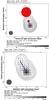 |
Fig. A.1
Example of 43 GHz VLBI images of S5 0716+714 observed on January 10, 2010 resolved with a beam size of 0.1 mas (gray circle in the bottom left corner of maps). Contour maps are superimposed with Gaussian model-fit components (red circles in the top panel) and clean delta components (plus symbols in the bottom panel). The blue lines mark the inner jet orientation. |
| Open with DEXTER | |
© ESO, 2014
Current usage metrics show cumulative count of Article Views (full-text article views including HTML views, PDF and ePub downloads, according to the available data) and Abstracts Views on Vision4Press platform.
Data correspond to usage on the plateform after 2015. The current usage metrics is available 48-96 hours after online publication and is updated daily on week days.
Initial download of the metrics may take a while.