| Issue |
A&A
Volume 566, June 2014
|
|
|---|---|---|
| Article Number | A55 | |
| Number of page(s) | 23 | |
| Section | Interstellar and circumstellar matter | |
| DOI | https://doi.org/10.1051/0004-6361/201323270 | |
| Published online | 11 June 2014 | |
Online material
Appendix A: Model of the dust emission
We detail how we construct a map of the model of the dust emission that is spatially
correlated with the Hi emission. The model of the dust emission M is written as
 (A.1)where AH is a map at
resolution Nside
= 512 built from the correlation measure αν in Eq. (2), B is an offset map built
from ων in Eq. (3), and HI is the NHI template
for the Hi GASS data.
(A.1)where AH is a map at
resolution Nside
= 512 built from the correlation measure αν in Eq. (2), B is an offset map built
from ων in Eq. (3), and HI is the NHI template
for the Hi GASS data.
The AH and B maps are computed from the results of the dust-Hi correlation analysis over 15° diameter patches, sampled on HEALPix pixels with a resolution Nside = 32.
Specifically, at each frequency, AH and B maps are derived from the correlation measure and the offset maps (Sect. 3.1). Next we correct the correlation measures and the offsets for the CMB contributions, following the procedure presented in Appendix B. The offset map is also corrected for the CIB monopole using the values determined in Planck Collaboration XI (2014). Subsequently, we obtain the desired AH map by interpolating the map of correlation measures from Nside = 32 to 512 of the original data using a Gaussian kernel with a standard deviation equal to the 1.°8 pixel size at Nside = 32. This final AH map is a slightly smoothed version of the initial map of the correlation measures. We follow the same procedure to interpolate the map of offsets ων and get the desired B map.
The CMB anisotropies and the noise increase the uncertainty of the dust emissivity and dust model for ν ≤ 217 GHz. To reduce these uncertainties at these low frequencies, in Planck Collaboration XXX (2014) but not in this paper for which this is not necessary, we choose to extrapolate the 353 GHz model using the greybody function in Eq. (8) for the mean temperature of 19.8 K and the map of spectral indices from Sect. 5.
Appendix B: CMB contribution to correlation measures
Here is how we proceed to find the CMB contribution to the correlation measures, i.e. the α(CHI) term in Eq. (6) in units of thermodynamic (CMB) temperature. The correlation measures corrected for the CMB contributions are used in Sect. 6 to compute the mean SED averaged over all sky patches, and in Appendix A for the dust model.
We assume that the dust SED at 100 ≤ ν ≤ 353 GHz is well approximated by a greybody spectrum with the spectral indices βmm determined in Sect. 5 and the mean dust temperature of 19.8 K. For each sky patch, we perform a linear fit between the correlation measures at 100, 143, 217, and 353 GHz and the greybody SED normalized to unity at 353 GHz, with weights taking into account the uncertainties of the correlation measures. The slope of the fit is the dust emissivity at 353 GHz, while the offset is our estimate of α(CHI).
For comparison, we also quantify the cross-correlation between the CMB and the Hi map using the SMICA map presented in the Planck component separation paper (Planck Collaboration XII 2014). A histogram of the difference between the two values of α(CHI) for the 135 sky patches at Nside = 8 is presented in Fig. B.1. The standard deviation 0.7 μK per 1020 H cm-2 represents only 3% of the standard deviation of the α(CHI) values. We consider this percentage as our uncertainty factor δCMB on the CMB correction in Eq. (7). The mean difference (− 0.15 μK per 1020 H cm-2) is within the expected statistical error.
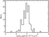 |
Fig. B.1
Histogram of the difference between two estimates of α(CHI) (the correlation measure between the CMB and the Hi template), found assuming a greybody spectrum for the dust emissivity or calculated with the SMICA CMB map. The standard deviation of the difference, 0.7 μK per 1020 H cm-2, is 3% of the standard deviation of α(CHI). |
| Open with DEXTER | |
Appendix C: Uncertainty of the dust emissivity
In this Appendix, we quantify the uncertainty of the dust emissivity. In the first subsection, we quantify the uncertainties from the correlation analysis. In the second, we assess the uncertainties associated with the definition of the Galactic Hi template that depends on the separation between Galactic and MS emission (see Sect. 2.2). Finally, we discuss uncertainties associated with subtraction of the zodiacal emission.
Appendix C.1: Correlation analysis
We describe how we estimate each of the contributions to σ(ϵH) (Eq. (7)), the uncertainty of the dust emissivity. At each Planck frequency, we obtain a noise map by computing and dividing by two the difference of the two maps made out of the first and second halves of each stable pointing period (Planck Collaboration VI 2014). For the DIRBE frequencies, we compute one Gaussian realization of the noise using the maps of data uncertainty. The noise maps are cross-correlated with the Hi template using the same mask and over the same sky patches. The standard deviation of the correlation measures over all the sky patches yields the noise contribution to σ(ϵH) at each of the Planck and DIRBE frequencies.
To estimate the additional contributions to σ(ϵH), we use sky simulations of the Galactic emission and CMB and CIB anisotropies. For the Galactic maps, we consider only dust emission. We compute dust maps by multiplying the Hi template with a Gaussian realization of the dust emissivity map as described in Appendix D. For the CMB and CIB anisotropies, we compute Gaussian realizations using the power spectra of the Planck best-fit CMB model in Planck Collaboration XV (2014), and of the CIB model at 857 GHz in Planck Collaboration XXX (2014). We scale CIB anisotropy simulations at 857 GHz to the full set of Planck-HFI and DIRBE frequencies using a mean SED of CIB anisotropies. This SED is a greybody fit to the Cℓ values at ℓ = 500 in Planck Collaboration XXX (2014). The spectral index is β = 1 and the temperature 18.3 K. We use 100 realizations of each of the Galactic, CIB and CMB maps. We cross-correlate each of the simulated maps with the Hi template using the same circular sky patches with 15° diameter as for the data analysis.
Each component is analysed separately from the others to estimate its specific contribution to the error budget. The uncertainty of the dust emissivity is quantified by comparing the emissivity derived from the correlation analysis with the mean value of the input emissivity map for each sky patch and each realization. For the CMB contribution, we use a fractional error δCMB of 3% from Appendix B. In Fig. C.1, the four contributions to the fractional error σ(ϵH) /ϵH are plotted versus frequency. The total uncertainty is the top solid line. We find that the Galactic residual contribution is dominant at ν> 217 GHz, and the CMB contribution is dominant at lower frequencies. The noise is significant for the 140 and 240 μm bands and for the lowest HFI frequencies.
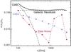 |
Fig. C.1
Fractional uncertainty (solid line) of the dust emissivities ϵH, normalized to the mean dust SED in Table 1. This total consists of contributions from Galactic residuals (black dashed line), noise (red dashed line with stars), CIB anisotropies (blue dotted line), and the CMB correction (black dash-dotted line). The Galactic residual contribution is dominant at ν> 217 GHz, and the CMB contribution is dominant at lower frequencies. |
| Open with DEXTER | |
These results depend on the size of the sky patches and on the angular resolution. To quantify this dependence, we repeat the analysis of the simulations for sky patches with diameters of 5° and . We find that the contributions from noise and CIB anisotropies scale with the inverse of the diameter, while the Galactic contribution remains roughly constant. The ratio between the CIB and Galactic contributions also increases when we use a template with higher angular resolution. These two effects contribute to make the CIB contribution to the uncertainties more important for the low column density fields in Planck Collaboration XXIV (2011) than in our study.
The simulations show that the uncertainties do not bias our estimates of the dust emissivity. At all frequencies, the mean emissivity averaged over all sky patches and all simulated maps is equal to the mean input value within statistical errors. We also find that the uncertainty of the mean emissivity is roughly independent of the size of the sky patches. The diameter that we use is thus not a critical aspect of our data analysis.
The Galactic and CIB contributions to the uncertainty of the dust emissivity are correlated between frequencies because variations of the SED of dust and CIB anisotropies are not taken into account. This reason is a simplification, but the data analysis does show that the residual maps, obtained after subtracting the dust model (Appendix A) from the data, are highly correlated between frequencies.
Appendix C.2: Galactic H I template
To assess the uncertainties associated with the separation of the Hi emission into Galactic and MS components (Sect. 2.2.2), we follow Planck Collaboration XXIV (2011) in correlating the Planck maps with three Hi maps for the low velocity gas (the original single tempate), and for the IVC and HVC components (Sect. 2.2.3). We perform this analysis over the same sky patches, using the same mask, as in our cross-correlation with a single Galactic Hi template (Sect. 3.3). We obtain dust emissivities for each of the three Hi velocity components. The emissivities for the low velocity component are very close to those reported in the paper for our analysis with a single template. For example, at 857 GHz the fractional difference between the two sets of values (the ratio between the difference and the mean value computed for each sky patch) has a 1σ dispersion of 1.1%, which is small compared to the main uncertainties in Fig. C.1. The mean difference between the two sets of values is negligible.
Appendix C.3: Subtraction of the zodiacal emission
We end this Appendix by comparing dust emissivities obtained from the analysis of Planck maps with and without subtraction of the zodiacal emission. We find that the differences are minor. For example, at 857 GHz, the fractional difference in correlation measures has a mean of zero and a standard deviation of 1.4%, which is one order of magnitude lower than the total uncertainty in Fig. C.1. The differences are highest, but still small (up to 5%), in sky patches near the southern Galactic pole that are close to the zodiacal bands and where the Galactic emission is faint.
Appendix D: Simulations of Galactic residuals to the dust- H I correlation
A histogram of the residuals with respect to the dust-Hi correlation is shown in Fig. 4. This Appendix describes how we simulate the Galactic contribution to the Gaussian part of this histogram. These simulations are used in Appendix C to estimate the contribution of Galactic residuals to the uncertainty of the dust emissivities, and in Planck Collaboration XXX (2014) to assess the associated contamination of the CIB power spectra.
It is beyond the scope of this appendix to explore fully the origin and nature of the Galactic residuals. We briefly discuss and quantify two possible contributions. (1) The residual Galactic emission could trace dust associated with diffuse ionized gas that is not spatially correlated with the Hi template. The column density of this warm ionized medium is known to account for ~20% of the total gas column density over the high latitude sky (Gaensler et al. 2008). (2) The Galactic residuals could arise from variations of the dust emissivity on angular scales smaller than the 15° diameter of the sky patches used in our correlation analysis. These variations would be the extension to small scales of the variations mapped by our correlation analysis (Fig. 3). These two contributions are not mutually exclusive: it is possible that each contributes. We do not consider residual emission from molecular gas, however, because the molecular fraction of the gas is known from UV observations to be low at column densities lower than 3 × 10²⁰ H cm-2 (Savage et al. 1977; Gillmon et al. 2006).
We produce sky simulations including each of these hypothetical contributions to the Galactic residuals and realizations of the CIB power spectrum. We process these simulated maps through the same correlation analysis as used on the Planck 857 GHz map. The simulations show that for each hypothesis we can match the amplitude and scatter of the values of σ857 in Fig. 7; however, it is only when the simulated maps include significant variations in the dust emissivity that the simulations match the systematic trend of σ857 growing with increasing NHI. We find that simulations can account for the main statistical properties of the Galactic residuals at 857 GHz when the map of variable dust emissivty is a Gaussian realization of a k-2.8 power spectrum, without needing any contribution from the warm ionized medium. The map of the dust emissivity is normalized to
reproduce the mean value and the standard deviation measured from the correlation of the 857 GHz map and the Hi template. We make multiple realizations of this specific model that are used in Appendix C and Planck Collaboration XXX (2014). The simulated maps at 857 GHz are scaled to other frequencies using the mean SED in Table 1. The simulations do not take into account the anti-correlation between the dust temperature and opacity.
© ESO, 2014
Current usage metrics show cumulative count of Article Views (full-text article views including HTML views, PDF and ePub downloads, according to the available data) and Abstracts Views on Vision4Press platform.
Data correspond to usage on the plateform after 2015. The current usage metrics is available 48-96 hours after online publication and is updated daily on week days.
Initial download of the metrics may take a while.