| Issue |
A&A
Volume 563, March 2014
|
|
|---|---|---|
| Article Number | A49 | |
| Number of page(s) | 25 | |
| Section | Extragalactic astronomy | |
| DOI | https://doi.org/10.1051/0004-6361/201322343 | |
| Published online | 06 March 2014 | |
Online material
Appendix A: Effective radius of the disk
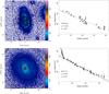 |
Fig. A.1
Left panels: color-scale representation of 1.5′× 1.5′ postage-stamp images extracted from the SDSS g-band data (in counts), centered on two CALIFA targets (UGC 00312 and NGC 7716), together with a set of ellipses (solid-black lines) representing the recovered shape at different isophotal intensity levels by the analysis described in the text. The last dashed red-black ellipse represents the 1σ isophotal intensity level over the background, adopting the median ellipticity and position angle to plot it. Right panels: surface brightness profiles derived for the considered galaxies on the basis of the corresponding isophotal analysis (gray solid circles), together with the best fit to an exponential profile for the portion of the surface brightness dominated by the disk (gray dashed line). For NGC 7716 a previous iteration of the fitting procedure is shown, before the rejection of those values dominated by the bulge (solid-line). |
| Open with DEXTER | |
In Sánchez et al. (2012b) we showed that the abundance gradient of the analyzed galaxies presents a common gradient up to ~2 re, when normalized to the effective radius of the disk (re). To repeat the same analysis for the CALIFA dataset included in this study, in addition to the abundances of the individual H ii regions, we need to derive this structural parameter for each galaxy.
The effective radius of the disk was derived from an analysis of the azimuthal surface brightness profile (SBP). To derive the SBP, we performed an isophotal analysis of the ancillary g-band images collected for the CALIFA galaxies (extracted from the SDSS imaging survey, York et al. 2000, and Paper I).
These images were created using the SDSSmosaic tool included in IRAF7 (Zibetti et al. 2009). SDSSmosaic takes the galaxy coordinates as input argument and downloads all the individual SDSS frames and the photometric information from the SDSS DR7 web site for all five bands. These frames are then stitched together, accurate astrometry is computed, and the photometric calibration is written into the header. After that, the background is subtracted from each scan by fitting a plane surface (allowing for linear gradient along the scan direction, constant in the perpendicular direction) outside a circle centered on the source. Finally, stripes are combined in a mosaic using the program Swarp (Bertin et al. 2002). The final mosaic contains the photometric zero point (P_ZP keyword) in mag per second of exposure time (EXPTIME keyword). We extracted postage-stamp images of 3′×3′ size, centered on the CALIFA targets, for the g-band mosaic images to derive the disk effective radius.
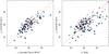 |
Fig. A.2
Left panel: distribution of the effective radius of the analyzed galaxies, derived from a growth curve analysis (i.e., the total light effective radius), as a function of the same effective radius derived by a similar growth curve analysis using the surface-brightness profiles derived using the ellipse task in IRAF. Right panel: distribution of the effective radius of the analyzed galaxies, derived from a growth curve analysis (i.e., the total light effective radius), as a function of the effective radius of the disk, derived from the exponential fitting to the surface brightness profile. In both panels, larger and bluer symbols correspond to earlier-type galaxies, while smaller and pinky/reddish ones correspond to later type galaxies. |
| Open with DEXTER | |
The isophotal analysis used the ellipse_isophot_seg.pl tool
included in the HIIexplorer package8).
Unlike to other tools, like ellipse included in IRAF, this tool
does not assume a priori a certain parametric shape for the isophotal distributions. The
following procedures were followed for each postage-stamp image: (i) the peak intensity
emission within a certain distance of a user defined center of the galaxy was derived.
Then, any region around a peak emission above a certain percentage of the galaxy
intensity peak is masked, which effectively masks the brightest foreground stars; (ii)
once the peak intensity is derived, the image is segmented in consecutive levels
following a logarithmic scale from this peak value, using the equation
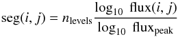 (A.1)where
seg(i,j) is the final segmented index at the pixel
(i,j), as an integer number; nlevels is the number of
selected levels of the isophotal analysis (100 in our case); flux(i,j)
is the intensity at the corresponding pixel (i,j) and
fluxpeak is the peak intensity at the center of the galaxy;
(iii) once the image is segmented in nlevels isophotal regions, for each of
them, a set of structural parameters was derived, including the mean flux intensity and
the corresponding standard deviation, the semi-major and semi-minor axis lengths, the
ellipticity, the position-angle, and the barycenter coordinates. These parameters are
intended to describe each isophote following an elliptical shape, but without performing
a direct fit, which is in principle more stable in lower S/N regimes. The lefthand panel
of Fig. A.1 illustrates the process, showing for
two particular objects a central section of 1.5′× 1.5′ of the postage-stamp images used
in this analysis, together with a set of ellipses plotted using the recovered shape
parameters for some particular isophotes.
(A.1)where
seg(i,j) is the final segmented index at the pixel
(i,j), as an integer number; nlevels is the number of
selected levels of the isophotal analysis (100 in our case); flux(i,j)
is the intensity at the corresponding pixel (i,j) and
fluxpeak is the peak intensity at the center of the galaxy;
(iii) once the image is segmented in nlevels isophotal regions, for each of
them, a set of structural parameters was derived, including the mean flux intensity and
the corresponding standard deviation, the semi-major and semi-minor axis lengths, the
ellipticity, the position-angle, and the barycenter coordinates. These parameters are
intended to describe each isophote following an elliptical shape, but without performing
a direct fit, which is in principle more stable in lower S/N regimes. The lefthand panel
of Fig. A.1 illustrates the process, showing for
two particular objects a central section of 1.5′× 1.5′ of the postage-stamp images used
in this analysis, together with a set of ellipses plotted using the recovered shape
parameters for some particular isophotes.
The isophotal segmentation (2nd step of the described procedure), was first introduced by Papaderos et al. (2002). Noeske et al. (2003) and Noeske et al. (2006) show that the surface-brightness profiles derived using this technique were very similar to those derived using more broadly adopted techniques, such as the 2D GALFIT code (Peng et al. 2002). We have adopted this isophotal annuli procedure in previous studies, e.g., Kehrig et al. (2012), Papaderos et al. (2013) and Mast et al. (2014). The improvement with respect to a pure isophotal segmentation was the additional derivation of the structural parameters for each isophotal region, described above (step iii).
The isophotal analysis provides an SBP, which is then analyzed to derive the required
effective radius. The righthand panel of Fig. A.1
shows two examples of the derived SBPs for those galaxies shown in the left panels. In
(Sánchez et al. 2012b), where all the galaxies
were clearly disk-dominated, the profiles were fitted using a pure exponential profile,
following the classical formula,
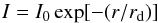 (A.2)where
I0 is the central intensity, and
rd is the disk scalelength (Freeman 1970), using a simple polynomial regression
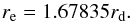
fitting. The scalelength was then used to derive the disk effective radius, defined as
the radius at which the integrated flux is half of the total one for a disk component by
integrating the previous formula and deriving the relation:
(A.2)where
I0 is the central intensity, and
rd is the disk scalelength (Freeman 1970), using a simple polynomial regression
fitting. The scalelength was then used to derive the disk effective radius, defined as
the radius at which the integrated flux is half of the total one for a disk component by
integrating the previous formula and deriving the relation:
 (A.3)In the current
study, the sample comprises galaxies of different morphological types. In many cases the
presence of a bulge prevents us from doing a direct exponential fitting for the complete
SBP. In those cases, the effective radius of the disk diverge from the effective radius
of the complete galaxy, defined as the semi-major axis encircling half of the light of
the galaxy.
(A.3)In the current
study, the sample comprises galaxies of different morphological types. In many cases the
presence of a bulge prevents us from doing a direct exponential fitting for the complete
SBP. In those cases, the effective radius of the disk diverge from the effective radius
of the complete galaxy, defined as the semi-major axis encircling half of the light of
the galaxy.
First, to illustrate that our isophotal analysis provides consistent results with more classical analysis tools, we determined the effective radius using a classical growth-curve analysis, based both on our procedure and the surface-brightness analysis provided by the ellipse task included in IRAF. The latter analysis is part of the CALIFA sample characterization effort, which can be performed only in regular shaped targets (Walcher et al., in prep.). The lefthand panel of Fig. A.2 shows the comparison between both effective radii. Different sizes and colors are used to illustrate the morphological type of the galaxies, with smaller and pink symbols corresponding to later type galaxies, and bluer and larger symbols corresponding to earlier type ones. There is an almost one-to-one relation between both parameters, without any evident difference between different morphological types. The comparison of other shape parameters, such as the position angle or the ellipticity produce similar results.
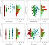 |
Fig. A.3
Top-left panel: distribution of the slopes of the abundance gradients as a function of the interaction stage of the galaxies, when the galactocentric distances are normalized to the effective radius derived by a growth curve analysis. The colors of the symbols and the corresponding histograms indicate three types of galaxies based on the interaction: (i) no signatures of interaction (red); (ii) galaxies with close companions and/or in an early interaction stage (green); and (iii) galaxies under clear collision or evolved mergers (blue). Top-right panel: similar distribution of slopes as a function of the morphological classification of the galaxies. The colors of the symbols and the corresponding histograms indicate three types of galaxies based on their morphology: (i) early spirals, SO-Sa (red); (ii) intermediate spirals, Sab-Sb (green) and (iii) late spirals, Sc-Sm (blue). Bottom-left panel: similar distribution of slopes as a function of the presence or absence of bars. The colors of the symbols and the corresponding histograms indicate three types of galaxies: (i) clearly unbarred (red); (ii) not clear if there is a bar or not (green) and (iii) clearly barred galaxies (blue). Bottom-right panel: similar distribution of slopes as a function of the absolute magnitude of the galaxies. The colors of the symbols and the corresponding histograms indicate three types of galaxies based on the luminosity: (i) luminous galaxies, Mg−SDSS < −20.25 mag (red); (ii) intermediate galaxies −19.5 < Mg−SDSS < −20.25 mag (green) and (iii) faint galaxies Mg−SDSS > −19.5 mag (blue). The size of the symbols are inversely proportional to the derived error in the slope for all the panels. |
| Open with DEXTER | |
To derive the disk effective radius it is required to fit that the outer portion of the SBP clearly dominated by an exponential disk. As illustrated in the righthand panels of Fig. A.1, in some cases there is almost no deviation from an exponential disk over the full spatial range covered by the SBP (e.g., UGC 00312). However, in other cases there is a clear deviation in the inner regions due to the presence of a bulge (e.g., NGC 7716). To minimize the effect of the bulge in this derivation we perform an iterative procedure, in which the SBP, represented in surface brightness magnitudes, was fitted with a linear regression. In each stage of the iteration, the brightest value of the SBP was removed, and the regression was repeated. The iteration stops when only half of the original values remains in the SBP. From the set of regressions it was adopted that one with the highest correlation coefficient between the semi-major axis and the surface brightness magnitude.
The procedure was tested visually, as illustrated in Fig. A.1, showing that it provides a good fit for the linear regime (i.e., the disk-dominated regime), excluding in most of the cases the central regions dominated by a bulge. Obviously, the procedure works better for those galaxies that are still dominated by disk in most of the SBP, and provides the worst results for those ones dominated by a bulge. However, this would be a general limitation to any other proposed method with the same aim.
The righthand panel of Fig. A.2 shows the comparison between the effective radius derived using the growth-curve method and the disk effective radius extracted from the iterative fit of the SBP. The size and color of the symbols represent the same morphological segregation shown in the lefthand panel. As expected the late-type galaxies, which are disk-dominated, are clustered closer to the one-to-one relation, while most of the earlier-type ones with brighter bulges are shifted toward larger disk effective radii.
Appendix B: Dependence of the results on the derivation of the disk effective radius
The main result described throughout the current study is that all undisturbed galaxies with a disk present a similar radial abundance gradient with a characteristic slope, when the galactocentric distances are normalized to the disk effective radius. This characteristic slope seems to be independent of other properties of the galaxies, such as morphological types, presence of a bars and absolute magnitudes or stellar masses. However, this result relies on the definition of the disk effective radius and its derivation, based on the surface brightness profile analysis described in the previous section.
The disk effective radius is a non-standard scalelength, which we have introduced to characterize the size of the disk in galaxies with different morphologies. Therefore, it is important to illustrate how our results are affected by this adopted normalization of the radial distances. To do so we repeat the analysis using the standard effective radius derived using the growth-curve analysis (re,GC) to normalize the abundance gradients, instead of the disk effective radius. As already indicated, the growth curve effective radius has been derived independently using different procedures providing, reliable and consistent results (Fig. A.2, left panel).
Figure A.3 shows the distribution of the new slopes obtained when normalizing to these effective radius along the same structural parameters of the galaxies shown in Fig. 8. Even though individual slopes change, in particular for the galaxies of earlier type, all the results described in Sect. 4.2 remain valid:
-
Galaxies with evidence of interaction or ongoing a clear merging process present an oxygen abundance gradient flatter than those without any clear evidence of interaction. The difference is statistically significant, both using KS- or a t-test for the different distributions. The characteristic slope for non-interacting galaxies it is not affected by the selection of the normalization radius, with a mean value of αO/H = −0.11 ± 0.09 dex/re (although the dispersion suffer a slight increase).
-
The average slope for earlier type galaxies is slightly flatter when normalizing by re,GC, instead of the disk re: αO/H,Sa/S0 = −0.06 ± 0.08 dex/re,GC instead of αO/H,Sa/S0 = −0.08 ± 0.08 dex/re. However, there is no significant different in the distribution of slopes, using either a KS- or a t-test analysis.
-
Neither the average slopes nor the distribution of slopes change significantly depending on the presence or absence of a bar in the galaxies. The use of the total or disk effective radius seems to be irrelevant for comparing of abundance gradients for barred an unbarred galaxies.
-
The abundance gradient slopes normalized by re,GC do not present any dependence on the absolute magnitudes, the stellar masses, or the concentration indices of the galaxies.
In summary, although the slopes of the individual gradients for each galaxy change when normalizing by the disk re or the re,GC, in general the statistical results are basically the same. The main effect, as expected, is found in the slope of the earlier type galaxies (Sa/S0), that present slightly flatter gradients. This is expected, since for these galaxies the disk re is larger than the growth curve one, due to the presence of a bulge. For those galaxies the derivation of the disk re is also more complicated, for the same reason. However, that the slope of the abundance gradient for these galaxies becomes more similar to the one derived for the latter type ones when using the disk effective radius, indicates that (i) the use of this radius provides a better characterization for the gradient and (ii) the metal enrichment seems to be clearly dominated by the growth of the disk, rather than other non-secular processes.
© ESO, 2014
Current usage metrics show cumulative count of Article Views (full-text article views including HTML views, PDF and ePub downloads, according to the available data) and Abstracts Views on Vision4Press platform.
Data correspond to usage on the plateform after 2015. The current usage metrics is available 48-96 hours after online publication and is updated daily on week days.
Initial download of the metrics may take a while.