| Issue |
A&A
Volume 562, February 2014
|
|
|---|---|---|
| Article Number | A47 | |
| Number of page(s) | 25 | |
| Section | Extragalactic astronomy | |
| DOI | https://doi.org/10.1051/0004-6361/201322011 | |
| Published online | 04 February 2014 | |
Online material
Stellar population properties.
Appendix A: Structural parameters: Half-light radius
To compare the spatial distribution of any given property in galaxies which are at different distances, the 2D maps need to be expressed in a common metric. We chose the half-light radius (HLR). To compute the HLR, we collapse the spectral cubes in the rest-frame window 5635 ± 45 Å, derive the isophotal ellipticity and position angle, and then integrate a curve of growth from which we derive the HLR. In some galaxies, the integrated image may contain masked regions at the position where the original cube contains foreground stars or some other artifacts (see Cid Fernandes et al. 2013 for further explanations) which may affect the estimation of the different parameters, including the HLR. To correct for these missing data, we build an average surface brightness radial profile for each galaxy using circular apertures. This profile is used to estimate the surface brightness of the spaxels masked in the original cube, assuming a smooth change of surface brightness between the missing data and the averaged values of their near neighbors at the same distance. This reconstructed flux image is used to derive the ellipticity and position angle of the aperture, and to obtain the average azimuthal radial profiles of the stellar population properties. These structural parameters are defined and obtained as follows:
-
Galaxy center: we take as the galaxy center the peak flux position. This definition is correct for most of the galaxies, except for the irregular galaxy CALIFA 475 (NGC 3991), where the maximum flux is well outside of the morphological center.
-
Ellipticity and position angle: the flux-weighted moments of the 5635 Å image are used to define the ellipticity and position angle (Stoughton et al. 2002). The reconstructed flux image is used to calculate the so-called Stokes parameters in order to obtain the ellipticity and position angle at each radial distance. The values, however, are kept constant beyond 2 HLR, which are taken to define a unique elliptical aperture for each galaxy. The final values do not change significantly after an iteration, filling the missing data with the surface brightness profile resulting from adding the flux with the derived elliptical aperture, and then estimating again the Stokes parameters.
-
Half-light radius (HLR): for each galaxy, the reconstructed flux image is used to build the flux curve of growth and to obtain the half-light radius. The flux is integrated in elliptical apertures with a position angle and ellipticity defined as explained above. The semi-major axis length at which the curve of growth reaches 50% of its maximum value is defined as the half-light radius,
 .
.
For the sample analyzed here,  kpc, with a mean value of 4.6 kpc. These values are higher than the Petrosian radius
  (obtained from the SDSS data archive), as shown in Fig. A.1. However, the circularized size, defined as
  , where ϵ is the ellipticity, follows well the one-to-one line, as does the HLR obtained through curve of growth integrating in circular rings,
  . The linear fit, in fact, deviates from the one-to-one line, giving circular HLR that are on average 5% lower than . The outlier in the correlation is CALIFA 886 (NGC 7311), the central galaxy of a compact group. Given the morphology of the system, is probably overestimated.
Table 1 lists values obtained for our sample. In this paper we will use HLR to refer generally to this metric, whether it is computed in circular or elliptical geometry, unless the specific results depend on the actual definition (as in Sect. 7).
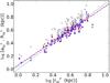 |
Fig. A.1
The Petrosian radius |
| Open with DEXTER | |

Appendix B: Quality of the spectral fits and uncertainties associated with evolutionary synthesis models
Appendix B.1: Quality of the spectral fits
All stellar population information used throughout this work comes from the starlight fits of the 98 291 individual spectra from 107 CALIFA data cubes. Here we illustrate these spectral fits with example spectra extracted from the nucleus and from a spaxel at 1 HLR for three different galaxies.
The top panels in Fig. B.1 show the nuclear spectra (black) of CALIFA 001 (IC 5376), CALIFA 073 (NGC 776), and CALIFA 014 (UGC 00312). The respective starlight fits are shown by the red line. Each panel also shows the Oλ − Mλ residual spectrum. Examples of fits for regions 1 HLR away from the nucleus are shown in the bottom panels.
As customary in full spectral fitting work, the fits look very good. In these particular examples the figure of merit  , defined as the mean value of | Oλ − Mλ | /Mλ (Eq. (6) in Cid Fernandes et al. 2013), is
  % (5.8%) for the nucleus (at 1 HLR) of IC 5376, 1.3% (5.8%) for NGC 776, and 1.6% (5.0%) for UGC 00312. The median values for the 107 galaxies are
  at the nucleus and 5.1% at R = 1 HLR. The SSP models used in these examples are from the GM base, built from evolutionary synthesis models by González Delgado et al. (2005) and Vazdekis et al. (2010), as summarized in Sect. 3. Very similar results are obtained with bases CB and BC.
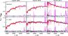 |
Fig. B.1
Example starlight fits for IC5376 (CALIFA 001, left), NGC 776 (CALIFA 073, middle), and UGC00312 (CALIFA 014, right). The top panels show the nuclear spectrum, while the bottom panels are for spaxels located at 1 HLR from the nucleus. Observed and synthetic spectra are shown in black and red lines, respectively. Masked regions (mostly emission lines) are plotted in magenta, and bad pixels are not plotted. Emission line peaks in the resdiual spectra were clipped for clarity. |
| Open with DEXTER | |
Appendix B.2: Uncertainties associated with using different SSP models
To evaluate to what extent the results of our spectral synthesis analysis depends on the choice of SSP models, we now compare properties derived with bases GM, CB, and BC. Since Cid Fernandes et al. (2014) have already performed this comparison for the same data analyzed here, we focus on comparisons related to specific points addressed in this paper.
First, we compare the results obtained for M∗. Figure B.2 shows the galaxy stellar mass distribution obtained with the CB and BC bases. The GM mass distribution (see Fig. 5a) is shifted to higher masses than CB and BC by ~0.27 dex, as expected because of the different IMFs (Salpeter in GM and Chabrier in CB and BC). The Salpeter IMF used in GM models has more low mass stars than the Chabrier function used in CB and BC, implying larger initial masses for the same luminosity. In addition, for the Salpeter IMF about 30% of this mass is returned to the ISM through stellar winds and SNe, while for a Chabrier IMF this fraction is 45%. These effects end up producing differences of a factor of ~1.8 in the total mass currently in stars.
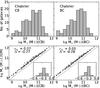 |
Fig. B.2
The galaxy stellar mass distributions obtained from the spatially resolved star formation history. The histograms show the results obtained with the bases GM, CB, and BC, from left to right, upper panels. The lower panels show the comparison of the galaxy stellar mass obtained with GM (vertical axis) and CB or BC (horizontal axis) for the 107 CALIFA galaxies. A one-to-one line is drawn in all the panels, as well as the best fit (dashed lines). The histogram inserted in each panel shows the differences in the log M∗ obtained with the base CB or BC with respect to GM. In the top-left corner of the panel, Δ is defined as CB – GM or BC – GM, and their dispersions are labeled. |
| Open with DEXTER | |
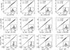 |
Fig. B.3
Comparison of stellar population properties obtained with bases GM (vertical axis) and CB or BC (horizontal axis) for the 107 CALIFA galaxies. A one-to-one line is drawn in all the panels, as well as the best fit (dashed lines). The histogram inserted in each panel shows the differences in the property obtained with the base CB or BC with respect to GM. In the top-left corner of each panel, Δ is defined as the mean CB − GM (or BC − GM) difference, and σΔ is the corresponding standard deviation. |
| Open with DEXTER | |
In the context of this paper, it is useful to compare the results for μ∗ and ⟨log age⟩L at the nucleus and at 1 HLR, as these allow us to estimate the uncertainties associated with the stellar mass surface density and age gradient due to the choice of SSP models. This is done in the top two rows of Fig. B.3, where values obtained with GM bases are plotted in the vertical axis, while CB- and BC-based estimates are in the horizontal. In all panels the labels Δ and σΔ denote the mean and rms of the difference of values in the y- and x-axis, and the histogram of these differences is shown in the inset panels.
The μ∗(0) and μ∗(1 HLR) values show the same 0.27 dex IMF-induced systematic differences seen in Fig. B.2. The dispersions in log μ∗ values are ~0.1 dex, much smaller than the ▽ log μ∗ gradients seen in Fig. 12. IMF factors shift log μ∗(0) and log μ∗(1 HLR) by the same amount. We thus conclude that SSP model choice has no significant impact on the μ∗ gradients discussed in this work.
Dispersions in the ⟨log age⟩L values are also of the order of 0.1 dex. One sees a small bias whereby the nuclei of mainly low mass galaxies are older with GM than CB by 0.05 dex, whereas the difference at 1 HLR is 0.02 dex. This would make ▽⟨log age⟩L~ 0.03 larger (i.e. a smaller gradient) with CB than with GM, a small effect which does not affect our conclusion that low mass galaxies show flat age radial profiles. The same small effect is found when comparing GM and BC ages.
Finally, we evaluate the effect of SSP choice on the half-mass and half-light radii dicussed in Sect. 7. We note that  depends on the spatial variation of the SFH (through the M/L ratio), while
  also depends on the radial variation of the stellar extinction. The bottom panels of Fig. B.2 show that the choice of SSP base has no significant impact upon the estimates of either HLR or HMR. Light-based sizes derived from GM, CB, and BC fits agree with each other to within ± 0.01 dex, while HMR have dispersion of 0.05 dex or less.
Appendix C: Missing mass in the CALIFA FoV
The main constraint in the sample selection for the CALIFA survey is a size7 isoAr < 79.2′′, only 7% larger than the PPAK FoV of 74′′. This implies that while some galaxies are completely enclosed within the FoV, others are somewhat larger. The question arises of how much stellar mass is left out of our stellar population synthesis analysis because it is out of the FoV. To estimate this “missing mass”, we proceed in the following manner, depicted in Fig. C.1 for the case of CALIFA 003. We use a 3′ × 3′ copy of the SDSS r-band image to compute and subtract the background around the galaxy; the distribution of the background residual is used to compute the edge of the galaxy as that enclosed above 1σ of the background (red contour in the figure). The missing flux (light blue in the top-right panel) is that contained within this contour and outside the CALIFA image; the points corresponding to this missing flux are represented in green in the radial profile in the bottom-left panel. From our population synthesis analysis of the CALIFA data cube, we compute the M/L ratio as a function of distance from the center of the galaxy (gray points in the bottom-right panel of the figure). The mean M/L value between 1.5 and 2.5 HLR is then used together with the missing flux to compute the missing mass outside the PPaK FoV. This is an approximate method, because we assume a constant value for the M/L in the outer parts of the CALIFA FoV, but the results are quite reliable, given that M/L has generally little or no gradient in these outer reaches, as can be seen in the bottom panels for the case of CALIFA 003.
The overall results for the missing mass are shown in the histogram of Fig. C.2; with a mean value of 8.63%, it shows a lognormal-type shape with a peak at ~5%.
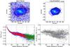 |
Fig. C.1
Upper-left panel: r-band SDSS image of NGC 7819 (CALIFA 003); a hexagon indicates the PPaK FoV, and a red contour shows the 1σ background. Upper-right panel: CALIFA image at 5635 Å; light blue shows the area of the galaxy outside the PPaK FoV, taken as that enclosed within the red contour in the left image minus the CALIFA image. The ellipses show the positions of 1 HLR and 2 HLR ( |
| Open with DEXTER | |

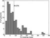 |
Fig. C.2
Histogram of the fraction of mass that is outside of the CALIFA FoV. The average value is marked by a vertical line. |
| Open with DEXTER | |
© ESO, 2014
Current usage metrics show cumulative count of Article Views (full-text article views including HTML views, PDF and ePub downloads, according to the available data) and Abstracts Views on Vision4Press platform.
Data correspond to usage on the plateform after 2015. The current usage metrics is available 48-96 hours after online publication and is updated daily on week days.
Initial download of the metrics may take a while.