| Issue |
A&A
Volume 558, October 2013
|
|
|---|---|---|
| Article Number | A110 | |
| Number of page(s) | 13 | |
| Section | The Sun | |
| DOI | https://doi.org/10.1051/0004-6361/201321348 | |
| Published online | 14 October 2013 | |
Online material
Appendix A: Flux weighting
Appendix A.1: Upstream conservation of flux
The flux of particles through a given cross-sectional area of the flux tube towards
the shock is given as  (A.1)which satisfies the
steady state requirement of
(A.1)which satisfies the
steady state requirement of  It is
noteworthy that although the mean direction of particles is in the negative
x-axis direction, we defined the total net flux across the shock as
being positive. We considered the shock to be an absorbing boundary, that is, the
distributions and fluxes represent particles that have yet to encounter the shock. The
particle flux, which is constant regardless of position
x1, is easily evaluated far from the shock, where only the
scattering process affects the angular distribution of the particles. The distribution
is assumed to be isotropic in the local plasma frame. Thus, sufficiently far upstream,
the flux is given by the form
It is
noteworthy that although the mean direction of particles is in the negative
x-axis direction, we defined the total net flux across the shock as
being positive. We considered the shock to be an absorbing boundary, that is, the
distributions and fluxes represent particles that have yet to encounter the shock. The
particle flux, which is constant regardless of position
x1, is easily evaluated far from the shock, where only the
scattering process affects the angular distribution of the particles. The distribution
is assumed to be isotropic in the local plasma frame. Thus, sufficiently far upstream,
the flux is given by the form
 (A.2)where
n∞ is the particle density and
f∞ the particle distribution at infinity.
(A.2)where
n∞ is the particle density and
f∞ the particle distribution at infinity.
At velocities
v < u1, all
particles travel towards the shock, and thus, information of the shock at
x1 = 0 cannot propagate into the upstream. The
distribution remains isotropic in the local plasma frame, and the differential flux
impacting the shock is simply  (A.3)Considering
particles with speeds
v > u1, the
picture becomes more complicated. Information of the shock can propagate against the
flow of plasma, because μv − u1 can be
positive. This means that the angular distribution of particles that have not yet
interacted with the shock becomes anisotropic, as the distribution
f(x1 = 0,v,μ) = 0 for
μv > u1, due to
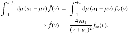
the absorbing boundary at the shock. However, at a distance of
x1 = 2λ, for instance, we can still
assume isotropy and take
f(2λ,v,μ) ≈ f∞(v),
so that
(A.3)Considering
particles with speeds
v > u1, the
picture becomes more complicated. Information of the shock can propagate against the
flow of plasma, because μv − u1 can be
positive. This means that the angular distribution of particles that have not yet
interacted with the shock becomes anisotropic, as the distribution
f(x1 = 0,v,μ) = 0 for
μv > u1, due to
the absorbing boundary at the shock. However, at a distance of
x1 = 2λ, for instance, we can still
assume isotropy and take
f(2λ,v,μ) ≈ f∞(v),
so that  (A.4)is valid for
all velocities including
v > u1. In this
flux, particles with
μv > u1 cause a
negative contribution to the net flux, because they propagate outwards across the flux
tube cross-section surface at x1 = 2λ.
(A.4)is valid for
all velocities including
v > u1. In this
flux, particles with
μv > u1 cause a
negative contribution to the net flux, because they propagate outwards across the flux
tube cross-section surface at x1 = 2λ.
For the purpose of constructing a semi-analytical model of particle injection at high
particle speeds, we simplified the anisotropies of the particle distribution at the
shock. We assigned the modified differential flux of particles with
v > u1 at the
shock as 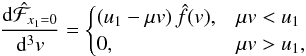 (A.5)where
 is a scaled distribution function yielding the correct total net flux, that is,
 for v < u1, but
for v > u1,
for v < u1, but
for v > u1,
 Thus,
for the particles that have not yet interacted with the shock, we find
Thus,
for the particles that have not yet interacted with the shock, we find 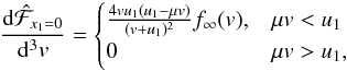 (A.6)valid
for particles of speed
v > u1. This
accounts for the absorbing boundary at the shock whilst maintaining the conservation
of total flux at a given particle speed v.
(A.6)valid
for particles of speed
v > u1. This
accounts for the absorbing boundary at the shock whilst maintaining the conservation
of total flux at a given particle speed v.
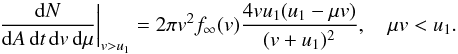
For Monte Carlo simulations, the same consideration of flux conservation must be
made. The flux, that is, the total amount of particles encountered by the shock within
time dt, is formulated as
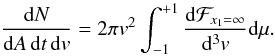 (A.7)For
particles of speeds
v < u1, the
whole population is advected towards the shock, meaning that no information of the
approaching shock can reach the particle distribution before impact. Thus, for these
particles, the differential flux, extended to encompass all pitch-angles, can be
written as
(A.7)For
particles of speeds
v < u1, the
whole population is advected towards the shock, meaning that no information of the
approaching shock can reach the particle distribution before impact. Thus, for these
particles, the differential flux, extended to encompass all pitch-angles, can be
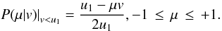
written as 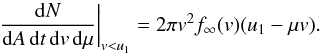 (A.8)Thus,
the probability of a particle with speed v exhibiting pitch-angle
μ when impacting the shock is given as
(A.8)Thus,
the probability of a particle with speed v exhibiting pitch-angle
μ when impacting the shock is given as
 (A.9)This
can be integrated to find the cumulative distribution function for a value of
μ as
(A.9)This
can be integrated to find the cumulative distribution function for a value of
μ as 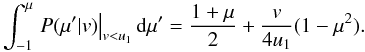 (A.10)From
this, the Monte Carlo randomisation formula for μ can be solved as
(A.10)From
this, the Monte Carlo randomisation formula for μ can be solved as
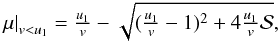 (A.11)where
μ receives values from the range
−1 < μ ≤ + 1 and
(A.11)where
μ receives values from the range
−1 < μ ≤ + 1 and
 is a uniformly distributed random number in the range [0,1).
For particles with speeds v > u1, information of the propagating shock can extend into the upstream, affecting the incident particle pitch-angle distribution. Thus, we initialised the particle distribution in the upstream of the shock at a distance of x1 = 2λ, and allowed particles to convect towards the shock. This resulted in a realistic pitch-angle distribution at x1 = 0+, without having to resort to flux modification (Eq. (A.6)).
This pre-propagation is limited to the region x1 ∈ [0,2λ] with particles initialised isotropically at values μ < u1/v. As the total population is advected towards the shock, all particles that escape to x1 > 2λ will eventually return to the initialisation boundary of x1 = 2λ, isotropised in the fluid frame. Thus, particles escaping to the upstream can be simply re-initialised at that position.
The distribution of pitch-angles μ for a given speed
v, limiting the valid pitch-angle range to values
 and normalising the total probability to 1, is
 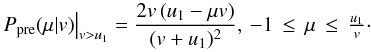 (A.12)This
will result in the shock-incident flux
(A.12)This
will result in the shock-incident flux
 (A.13)Using Eq.
(A.12), the Monte Carlo
randomisation formula for μ can be solved (similar to Eq. (A.10)) as
(A.13)Using Eq.
(A.12), the Monte Carlo
randomisation formula for μ can be solved (similar to Eq. (A.10)) as 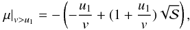 (A.14)where
μ receives values from the range
(A.14)where
μ receives values from the range
 .
.
Appendix B: Analytical injection thresholds
Appendix B.1: Reflection threshold
In attempting to determine particle injection, we can solve certain seed particle
speed thresholds. A particle is reflected (see Eq. (9)), and thus, injected, if  (B.1)The right-hand side
(RHS) of the equation is constant. Through roots of derivatives of the left-hand side
(LHS), we can find LHS maxima at
(B.1)The right-hand side
(RHS) of the equation is constant. Through roots of derivatives of the left-hand side
(LHS), we can find LHS maxima at  if
if
 ,
or μ = 1, if
,
or μ = 1, if  .
Thus, if ,
the LHS maximum is given as
.
Thus, if ,
the LHS maximum is given as 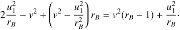 (B.2)This results
in no possibility of reflection, if
u1/rB < v < vR1,
where
(B.2)This results
in no possibility of reflection, if
u1/rB < v < vR1,
where 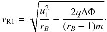 (B.3)If
,
the LHS has a maximum value of
2vu1 − v2.
This results in no possibility of reflection, if
v < vR2, where
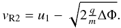
(B.3)If
,
the LHS has a maximum value of
2vu1 − v2.
This results in no possibility of reflection, if
v < vR2, where
 (B.4)The LHS minimum is
found at μ = −1. With these shock and solar wind parameters, there
exists no valid speed v for which this value of the LHS would be
positive. Under these circumstances, no seed particle speed v results
in certain reflection, regardless of pitch-angle μ.
(B.4)The LHS minimum is
found at μ = −1. With these shock and solar wind parameters, there
exists no valid speed v for which this value of the LHS would be
positive. Under these circumstances, no seed particle speed v results
in certain reflection, regardless of pitch-angle μ.
Appendix B.2: Threshold for return from the downstream
To split the transmitted particle population into portions with either possible or
impossible injection, we examined Eqs. (10)and (11)to find
 (B.5)We
found the maxima of downstream speed v′ for a given
v, because this can result in an injection velocity threshold.
Maxima for v′ can be found at μ = −1
and μ = + 1 or by solving the roots of the derivative of
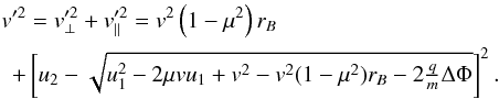
v′(μ). Assigning
(B.5)We
found the maxima of downstream speed v′ for a given
v, because this can result in an injection velocity threshold.
Maxima for v′ can be found at μ = −1
and μ = + 1 or by solving the roots of the derivative of
v′(μ). Assigning
 (B.6)and finding
the first derivative for v′2 gives
(B.6)and finding
the first derivative for v′2 gives 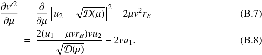 Solving
the roots provides an extremum, if μ ∈ (−1, + 1)
and if
Solving
the roots provides an extremum, if μ ∈ (−1, + 1)
and if 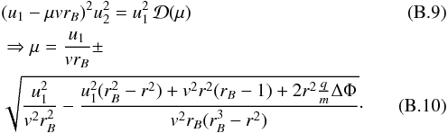 If
If
 holds true, only the solution with the minus sign is of interest. These, in addition
to the possible extrema at μ = −1 and μ = + 1,
result in several possible threshold velocities.
holds true, only the solution with the minus sign is of interest. These, in addition
to the possible extrema at μ = −1 and μ = + 1,
result in several possible threshold velocities.
Appendix B.2.1: Extrema at μ =-1 and μ = + 1
The possible downstream velocity extrema at μ = −1 and
μ = + 1 can be solved by refining Eq. (B.5). Formulating this as the threshold
for no injection results in
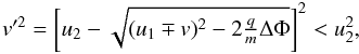 (B.11)where the term
inside the square root is positive for all transmitted particles. Thus, a
transmitted particle can return to the upstream only if
(B.11)where the term
inside the square root is positive for all transmitted particles. Thus, a
transmitted particle can return to the upstream only if
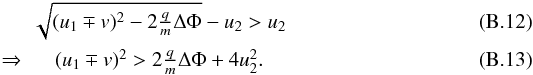 For
particles with
v > u1,
injection is always possible. For particles with
v < u1, we
found the additional requirements of
For
particles with
v > u1,
injection is always possible. For particles with
v < u1, we
found the additional requirements of 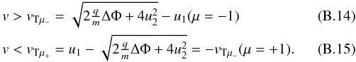 For
our parameters, only vTμ−
provides a valid condition for injection.
For
our parameters, only vTμ−
provides a valid condition for injection.
Appendix B.2.2: Extrema at μ ≠ ± 1
Solving the thresholds speeds for the one or two extrema given in Eq. (B.8)in an analytical fashion does not result in easily applicable equations. However, solving the velocity thresholds for these extrema in a numerical fashion revealed valid extrema only at shock-normal angles θBn ≤ 4°. At these shock-normal angles, the existing extrema at μ = ± 1 already allow theoretical return of particles regardless of their speed. Thus, these extrema do not affect the found particle return speed thresholds. However, in a more general case, they cannot be ignored.
Appendix C: Statistical handling of uninjected particles
In Sect. 7, we presented a method for estimating
the capability of a shock to inject particles using Monte Carlo simulations. In our
method, we propagated the particle in the downstream until it was either injected into
the upstream, or the cumulative probability of return at the downstream boundary fell
below 10-6 and it was removed from the simulation as an uninjected particle.
For some shock parameters, however, this method will result in very low statistics for
the injected particles. To improve the statistical accuracy, we used the fact that
successes and failures – injections and non-injections – are distributed according to a
negative binomial distribution. When the numbers of successes, ℛ, and failures,
 ,
are known, the probability for success
,
are known, the probability for success  can be evaluated using the minimum-variance unbiased estimator (see, e.g., Lehmann & Casella 1998), which gives
 (C.1)It should be
noted, however, that the actual probability of injection for a particle is
(C.1)It should be
noted, however, that the actual probability of injection for a particle is
 (C.2)
(C.2)
where Ps is the injection probability associated with the last encountered success.
To evaluate the unbiased estimator, we randomised particles in groups. For each
particle within the group, the newly randomised values of v and
μ were used to test the particle for reflection, as explained in
Sect. 5.1. Reflected particles were considered
successes and have Ps = 1. Non-reflected particles are
transmitted to the downstream, with v′ and
μ′ calculated according to Eqs. (10)and (11). They were then followed in the downstream, as described in
Sect. 7, until they were either injected,
incrementing ℛ, or considered uninjected, incrementing
.
This was continued until ℛ = 5. The last particle of the group was then injected with
the probability Pinj.
As a precaution against excessively low success probabilities, the group size was
limited to  .
If this limit was reached and at least two successes were encountered, the values of
ℛi and
.
If this limit was reached and at least two successes were encountered, the values of
ℛi and  associated with the last encountered success were used to calculate
.
If the tests resulted in only 0 or 1 success, the group was considered to result in no
injection.
associated with the last encountered success were used to calculate
.
If the tests resulted in only 0 or 1 success, the group was considered to result in no
injection.
With these methods, the injected weight of the Monte Carlo particle was found to be Winj = WseedPinj, where Wseed is the representative weight of upstream seed particles assigned to this group, and was found based on the plasma density. The total injected weight was then used to calculate the particle flux.
© ESO, 2013
Current usage metrics show cumulative count of Article Views (full-text article views including HTML views, PDF and ePub downloads, according to the available data) and Abstracts Views on Vision4Press platform.
Data correspond to usage on the plateform after 2015. The current usage metrics is available 48-96 hours after online publication and is updated daily on week days.
Initial download of the metrics may take a while.