| Issue |
A&A
Volume 556, August 2013
|
|
|---|---|---|
| Article Number | A115 | |
| Number of page(s) | 15 | |
| Section | The Sun | |
| DOI | https://doi.org/10.1051/0004-6361/201321629 | |
| Published online | 06 August 2013 | |
Appendices
Appendix A: The flat-field correction
Especial care must be taken with the flat-fielding procedure. At the SST, the flat-field data are acquired while the telescope moves in circles around solar disk center, accumulating ≈1000 images per wavelength and polarization state. Effectively, the data represent a temporal and spatial average of quiet-Sun data at solar disk center. Therefore, it is reasonable to assume that the observed line profile at each pixel should be almost identical, except for the dirt, wavelength dependent fringes and the prefilter transmission, that can change across the FOV.
The telecentric configuration used in CRISP is optimal to achieve high spatial-resolution observations, although the instrumental transmission profile is not constant across the field-of-view (FOV). Pixel-to-pixel wavelength shifts (cavity errors) are present due to imperfections in the surface of the etalons that cannot be infinitely flat. Additionally, imperfections in the coating of the etalons produce reflectivity variations across the FOV that change the width of the transmission profile (reflectivity errors).
These effects become obvious when a spectral line is present at the observed wavelength, producing intensity fluctuations across the FOV that correlate tightly with the cavity errors and, less obviously, with variations in the reflectivity.
While these instrumental effects are permanently anchored to the same pixels on the camera, solar features are moved around by differential seeing motions, however, the MOMFBD code is only able to process data where the intensity at any given pixel, is strictly changing due to atmospheric distortion. To overcome this problem Schnerr et al. (2011) proposed a strategy to characterize CRISP and prepare flat-field images that allow to reconstruct the data.
Their idea is founded on the assumption that each pixel observed the same quiet-Sun profile during the flat-field data acquisition. To remove the imprint of the quiet-Sun profile from each pixel, an iterative self-consistent scheme is used to separate the different contributions to the intensity profile at each pixel, which we summarize in the following lines. To reproduce the observed profile on a pixel-to-pixel basis, they assume that the intensity at each pixel can be expressed as,  (A.1)where Iobs is the observed profile at a given pixel, λ is the wavelength, IQS is the estimate of the spatially-averaged quiet-Sun profile, T is a theoretical CRISP transmission profile, c0 is a multiplicative factor that scales the entire profile and c3 accounts for shifts of the prefilter. ech and erh represent the high resolution etalon cavity error and reflectivity error respectively. The ∗ stands for a convolution operator.
We simplify their strategy, by assuming constant reflectivities across the FOV. Neglecting the effect of reflectivity errors works particularly well in broad-lines like the λ8542, given that the transmission profile is relatively narrow compared to the Doppler width of the line. It also reduces the time required to compute the fits, from hours to minutes on a single CPU, as no convolutions are required any longer. We also allowed to include two more terms to the prefilter polynomial, given that at this wavelength there are fringes that change as a function of wavelength, introducing some distortion in the profiles.
Figure A.1 (lower panel) illustrates a density map, where the profiles from all pixels have been divided by c0(1 + c3λ + c4λ2 + c5λ3) and shifted to the correct wavelength. The best estimate of the quiet-sun profile is plotted with a blue line. A tight correlation means that our model is able to reproduce the observed profiles, despite the simplifications applied to the original model by Schnerr et al. (2011). A cavity-error map is also shown in Fig. A.1
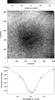 |
Fig. A.1
Top: map of the FPI cavity errors in units of wavelength shift. Bottom: density plot of all pixels in the summed flat-field data (orange clouds) that have been shifted to the correct wavelength and corrected for the different contributions in the model. The blue line is the average line profile described by a spline curve and closely resembles a disk center quiet Sun atlas profile. |
| Open with DEXTER | |
Appendix A.1: The CCD backscatter problem
The back-illuminated Sarnoff CAM1M100 CCD cameras used in the CRISP instrument allow to acquire 35 frames-per-second, freezing atmospheric motions during each acquisition. These cameras work particularly well in visible light, but their efficiency decreases steeply in the infrared.
Above approximately 7000 Å, the CCD becomes semi-transparent and the images show a circuit pattern that is not present at other wavelengths. de la Cruz Rodriguez (2010) explains a way to overcome this issue and properly apply the flat-field correction to the data. Furthermore, the images show a circuit-like pattern that cannot be removed by traditional dark-field and flat-field corrections, as illustrated in Fig. A.2 (top panel). Examination of pinhole data and flat-fielded data shows that:
-
1.
there is a diffuse additive stray-light contribution in the wholeimage;
-
2.
the stray-light contribution is much smaller in the circuit pattern and the gain appears to be enhanced.
These problems can be explained by a semi-transparent CCD with a diffusive medium behind it, combined with an electronic circuit located right behind the CCD that is partially reflecting and therefore also less transparent to the scattered light. Under normal conditions an image recorded with a CCD, Io, can be described in terms of the dark-field (D), the gain factor (Gf) and the real image (Ir): 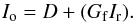 (A.2)However, in the infrared we need a more complicated model:
  (A.3)where f represents the overall fraction of light absorbed by the CCD, Gb is the gain for light illuminating the CCD from the back which should account for the electronic circuit pattern. In the following, we refer to Gb as backgain. P is a point spread function (PSF) that describes the scattering properties of the dispersive screen. In the backscatter term we assume that (1 − f)GfIrGb is transmitted to the diffusive medium where it is scattered. A fraction of the scattered light returns to the CCD, passing again through the circuit. The sketch in Fig. A.3 shows a schematic representation of the structure of the camera and the path followed by the light beam.
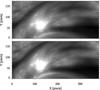 |
Fig. A.2
Top: subfield from an individual acquisition, where traditional dark-current and flat-field corrections have been applied. An electronic circuit pattern from the CCD chip is visible in the background. Bottom: same subfield, backscatter corrected. |
| Open with DEXTER | |
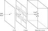 |
Fig. A.3
Sketch showing a conceptual model of the camera. The dark arrows indicate the incoming light beam from the telescope and the gray arrows represent the back-scattered light that returns to the CCD. |
| Open with DEXTER | |
To obtain the real intensity Ir, the PSF P, the back-gain Gb and the front-gain Gf must be known. The transparency factor is assumed to be smooth because the properties of the dispersive screen seem to be homogeneous across the FOV. This allows us to include f in the front and the back gain factors  so Eq. (A.3) becomes:
  (A.4)This problem is linear and invertible, but a direct inversion would be expensive, given the dimensions of the problem. A numerical approach can be used to iteratively solve the problem. We define
  (A.5)The back gain Gb′ is assumed to be 1 for every pixel in the first iteration. Furthermore, we assume that the product Gf′Ir can be estimated from Eq. (A.2) ignoring back scattering, i.e., Gf′Ir ≈ Io − D. These values are of the same order of magnitude as the final solution, and therefore correspond to a reasonable choice of initialization:
  (A.6)We assume rotational symmetry to construct the 2D PSF P, which is parameterized by placing node points along the radial component. The latter are connected by straight lines in logarithmic scale. To estimate the initial guess of the node points we use an angular average obtained from a pinhole image. The small diameter of the pinhole only allows to estimate accurately the central part of the PSF. The wings of our initial guess are extrapolated using a power-law. The estimate of Gf′Ir is then
 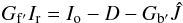 (A.7)which can be used to compute a new estimate Ĵ. This new value of Ĵ is used to improve our estimate of Gb′, by applying the same procedure to images that contain parts being physically masked (Ir = 0), as in Fig. A.4. In the masked parts where Ir ≡ 0 we have,
  (A.8)so the back-gain can be computed directly:
 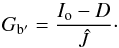 (A.9)Thus, every pixel must have been covered by the mask at least once in a calibration image in order to allow the calculation of the back-gain. With the new Gb′ we can recompute a new estimate of Gf′Ir. This procedure, enclosing Eqs. (A.7)−(A.9) is iterated, until Gf′Ir and Io are consistent.
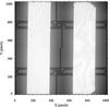 |
Fig. A.4
Calibration data acquired to infer the backgain and the PSF describing the backscatter problem. The dark areas are physically masked on the focal plane of the telescope. The color scale is saturated to enhance the CCD chip pattern. |
| Open with DEXTER | |
We now need to specify a measure that describes how well the data are fitted by the estimate of P and Gb′(P). Since both Gf′Ir and Gb′ are computed based on self-consistency, we iteratively need to fit only the parameters of the PSF. We assume that the PSF is circular-symmetric and apply corrections to the PSF at node points placed along the radius.
We use Brent’s Method described by Press et al. (2002) to minimize our fitness function. This algorithm does not require the computation of derivatives with respect to the free parameters of the problem. When the opaque bars block a region of the CCD, an estimate of the back gain can be calculated for a given PSF according to Eq. (A.9). In our calibration data, the four bars of width L are displaced 0.5 L from one image to the next. This overlapping provides two different measurements of the back gain on each region of the CCD. However, as the location of the bars changes on each image, the scattered light contribution is different for each of these measurements of the back gain. Our fitness function minimizes the difference between these two measurements of the back gain. Note that two nested iterative loops are needed to compute the parameters of the PSF. The inner loop is used to compute a self-consistent value of Gf′Ir for any given PSF P, whereas in the outer loop the parameters of a guessed PSF are fitted to compensate for the backscatter problem. We have summarized the work flow in Fig. A.5.
Having thus obtained the PSF P and the back-gain Gb′, we obtain Gf′ by recording conventional flats and assuming Ir is a constant in order to obtain Gf′ from Eq. (A.4).
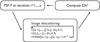 |
Fig. A.5
Work flow of out iterative scheme to fit the parameters of the backscatter PSF. The scheme has two nested iterative schemes, the inner loop is used to obtain the descattered image (Gf′Ir) for each set of guessed PSF parameters (the outer loop). |
| Open with DEXTER | |
Appendix B: The SST polarization model at λ854 nm
The optical path of the SST, from the 1m lens down to the cameras, contains optical elements that can polarize light. Therefore, polarimetric observations at the SST must be calibrated.
At the SST this calibration is split in two parts: the optical table and the turret. The former is calibrated daily, given that the observer can easily place a linear polarizer and a retarder to generate known polarization states, and analyze how the optical table changes the polarization (see van Noort & Rouppe van der Voort 2008, for further details).
The result is a modulation matrix Mtable that allows to convert the observed polarization states Ilc ≡ (Ilc0,Ilc1,Ilc2,Ilc3)T into Stokes parameters I ≡ (I,Q,U,V)T parameters, using a linear combination: 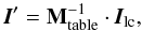 (B.1)where the prime symbol indicates that only the optical table has been calibrated.
In principle, if the telescope was built with non-polarizing elements then (I′,Q′,U′,V′) ≡ (I,Q,U,V), but this is not the case. The turret has mirrors and a lens that change the polarization properties of the incoming light. In fact, the polarizing properties of the turret change with the pointing. Therefore, a final transformation (Mtel) is needed to obtain telescope-polarization free Stokes parameters: 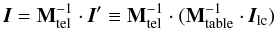 (B.2)Selbing (2010) studied the polarizing properties of the SST and proposed a model to characterize the telescope induced polarization at 630 nm. In this work, we use a similar model. Their work allows to compute Mtel based on the azimuth and elevation parameters of the telescope pointing.
Calibration images have been recorded during an entire day, using a 1-m polarizer mounted at the entrance lens of the SST. The polarizer rotates 360deg in steps of 5deg and several frames are acquired for each angle. These data are used to derive the parameters of the model proposed by Selbing (2010) at 854 nm. This model is already presented in de la Cruz Rodriguez (2010) and included here for completeness.
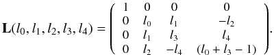
Each polarizing optical element of the telescope is represented with a Mueller matrix. L represents the entrance lens. The form of the lens matrix represents a composite of random retarders, so it demodulates the light without polarizing it. The reference for Q is aligned with the 1m linear polarizer axis and the values of the matrix are measured in that frame:
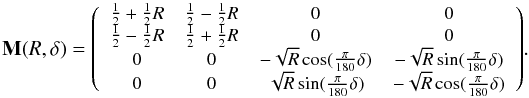
 Mirrors are noted with M and have two free parameters. Assuming a wave that propagates along the z-axis and oscillates in the x − y plane, the parameters are the de-attenuation term R between the xy components of the electromagnetic wave and the phase retardance δ produced by the mirror. This form of M assumes that Q is perpendicular to the plane of incidence:
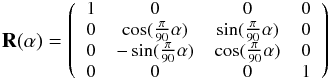
 Finally, R(α) corresponds to a rotation to a new coordinate frame:
 Selbing (2010) builds the telescope model using the Mueller matrix of each polarizing element, as a function of the azimuth (ϕ) and elevation (θ) angles of the Sun at the time of the observation (Eq. (B.3)). We have included the conversion factor from degrees to radians in the matrices, thus all the angles are given in degrees:
 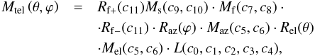 (B.3)where c1,2,...,11 are the parameters of the model, computed using a least-squares fit to the observed data. The fitted values are summarized in Table B.1.
Parameters of the telescope model obtained from calibration data at 8542 nm.
Note that the polarizer has a significant leak of unpolarized light at 854.2 nm. Using small samples of the sheets used to construct the 1-m polarizer, we have estimated the extinction ratio of the 1-m polarizer to be approximately 40%, so the parameters of the lens have been determined assuming that value.
The linear polarization reference is defined by the first mirror after the lens, however this is not very useful in practice because the turret introduces image rotation along the day. Instead, we use the solar north as a reference for positive Q by applying an extra rotation to Mtel.
The full-Stokes Ca ii images in Fig. 2 have been calibrated using the telescope model described in this section.
Online material
Movie of Fig. 3 (Access here)
© ESO, 2013
Current usage metrics show cumulative count of Article Views (full-text article views including HTML views, PDF and ePub downloads, according to the available data) and Abstracts Views on Vision4Press platform.
Data correspond to usage on the plateform after 2015. The current usage metrics is available 48-96 hours after online publication and is updated daily on week days.
Initial download of the metrics may take a while.