| Issue |
A&A
Volume 552, April 2013
|
|
|---|---|---|
| Article Number | A96 | |
| Number of page(s) | 18 | |
| Section | Cosmology (including clusters of galaxies) | |
| DOI | https://doi.org/10.1051/0004-6361/201220724 | |
| Published online | 04 April 2013 | |
Online material
Appendix A: Mock quasar spectra
We have produced mock spectra in order to tune the analysis procedure and to study statistical uncertainties and systematic effects in the measured correlation function.
In some galaxy clustering studies (e.g. Anderson et al. 2012) the covariance matrix of the measured correlation function is obtained from mock data sets. In this case, it is crucial to have very realistic mocks with the right statistics.
In order to do so, we would need to generate several realizations of hydrodynamical simulations, with a large enough box to cover the whole survey (several Gpc3) and at the same time have a good enough resolution to resolve the Jeans mass of the gas (tenths of kpc). This type of simulations are not possible to generate with current technology, but luckily in this study the covariance matrix is obtained from the data itself, and the mock data sets are only used to test our analysis and to study possible systematic effects.
In the last few years there have been several methods proposed to generate simplified mock Lyman-α surveys by combining Gaussian fields and nonlinear transformations of the field (Le Goff et al. 2011; Greig et al. 2011; Font-Ribera et al. 2012). In this study we used a set of mocks generated using the process described in Font-Ribera et al. (2012), the same method used in the first publication of the Lyman-α correlation function from BOSS (Slosar et al. 2011).
The mock quasars were generated at the angular positions and redshifts of the BOSS quasars. The unabsorbed spectra (continua) of the quasars were generated using the Principal Component Analysis (PCA) eigenspectra of Suzuki et al. (2005), with amplitudes for each eigenspectrum randomly drawn from Gaussian distributions with sigma equal to the corresponding eigenvalues as published in Suzuki (2006) Table 1. A detailed description will be provided by Bailey et al. (in prep.), accompanying a public release of the mock catalogs.
We generated the field of transmitted flux fraction, F, that have a
ΛCDM power spectrum with the fiducial parameters  (A.1)where
h = H0/100 km s-1Mpc-1.
These values produce a fiducial sound horizon of
(A.1)where
h = H0/100 km s-1Mpc-1.
These values produce a fiducial sound horizon of
 (A.2)Here, we use the
parametrized fitting formula introduced by McDonald
(2003) to fit the results of the power spectrum from several numerical
simulations,
(A.2)Here, we use the
parametrized fitting formula introduced by McDonald
(2003) to fit the results of the power spectrum from several numerical
simulations,  (A.3)where
μk = k∥/k
is the cosine of the angle between k and the line of sight,
bδ is the density bias parameter,
β is the redshift distortion parameter,
PL(k) is the linear matter power
spectrum, and
DF(k,μk)
is a non-linear term that approaches unity at small k. This form of
PF is the expected one at small k in
linear theory, and provides a good fit to the 3D Lyα observations
reported in Slosar et al. (2011). We do not
generate a density and a velocity field, but directly create the Lyα
forest absorption field instead, with the redshift distortions being directly introduced
in the input power spectrum model of Eq. (A.3), with the parameter β that measures the strength of the
redshift distortion.
(A.3)where
μk = k∥/k
is the cosine of the angle between k and the line of sight,
bδ is the density bias parameter,
β is the redshift distortion parameter,
PL(k) is the linear matter power
spectrum, and
DF(k,μk)
is a non-linear term that approaches unity at small k. This form of
PF is the expected one at small k in
linear theory, and provides a good fit to the 3D Lyα observations
reported in Slosar et al. (2011). We do not
generate a density and a velocity field, but directly create the Lyα
forest absorption field instead, with the redshift distortions being directly introduced
in the input power spectrum model of Eq. (A.3), with the parameter β that measures the strength of the
redshift distortion.
To model the evolution of the forest with redshift, bδ varies with redshift according to bδ = 0.14 [(1 + z)/3.25] 1.9 (McDonald et al. 2006). The redshift distortion parameter is given a fixed value of βF = 1.4. The non-linear correction factor D(k,μk) is taken from McDonald (2003). The flux field was constructed by generating Gaussian random fields g with an appropriately chosen power spectrum (Font-Ribera et al. 2012) to which the log-normal transformation F = exp(−aeυg) is applied (Coles & Jones 1991; Bi et al. 1992; Gnedin & Hui 1996). Here a and υ are free parameters chosen to reproduce the flux variance and mean transmitted flux fraction (McDonald et al. 2006).
DLA’s were added to the spectra according to the procedure described in Font-Ribera & Miralda-Escud (2012).
Finally, the spectra were modified to include the effects of the BOSS spectrograph point spread function (PSF), readout noise, photon noise, and flux miscalibration.
Fifteen independent realizations of the BOSS data were produced and analyzed with the same procedures as those for the real data.
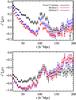 |
Fig. A.1
Effect of the continuum estimation procedure on the correlation function found with the mock spectra. The black dots are the average of monopole and quadrupole obtained with the 15 sets using the exact continua. The blue (red) dots show those obtained with the continuum estimation of method 1 (method 2) as described in Sect. 3.1 (3.2). |
| Open with DEXTER | |
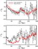 |
Fig. A.2
Comparison of the correlation function for the mock spectra and that for the data. The red dots show the mean of the 15 sets of mock spectra and the black dots show the data. |
| Open with DEXTER | |
We used the mock spectra to understand how our analysis procedure modifies the correlation function. Figure A.1 shows the average over 15 mocks of the reconstructed quadrupole and monopole using methods 1 and 2 (Sects. 3.1 and 3.2) and that reconstructed with the true continuum. The monopole and quadrupole for the two methods have a general shape that follows that found with the true continuum including the position of the BAO peak. However, both methods produce a monopole that becomes negative for 60 h-1 Mpc < r < 100 h-1 Mpc while the true monopole remains positive for all r < 130 h-1 Mpc. As discussed in Sect. 3.2, this result is due to the continuum estimation of the two methods which introduced negative correlations. For both methods, however, the BAO peak remains visible with a deviation above the “broadband” correlation function that is hardly affected by the distortion.
Figure A.2 presents ξ0(r) and ξ2(r) found with the data, along with the mean of 15 mocks. The figure demonstrates that our mocks do not perfectly reproduce the data. In particular, for r < 80 h-1 Mpc, the monopole is underestimated and the quadrupole overestimated. Since we use only peak positions to extract cosmological constraints, we only use the mocks qualitatively to search for possible systematic problems in extracting the peak position.
Appendix B: Results for a fiducial BOSS Lyα forest sample
The spectra analyzed here are all available through SDSS DR9 (Ahn et al. 2012), and the DR9 quasar catalog is described
by Pâris et al. (2012). A Lyα forest analysis requires many detailed choices about data selection and continuum determination. To aid community analyses and comparison of results from different groups, Lee et al. (2012b) has presented a fiducial BOSS Lyα forest sample that uses constrained PCA continuum determination (Lee et al. 2012a) and reasonable choices of masks for DLAs, BALs, and data reduction artifacts. Both the data selection and the continuum determination differ from those used here. Figure B.1 compares the Method 2 correlation function from this paper’s analysis to that obtained by applying the Method 2 weights and correlation measurement code directly to the continuum-normalized spectra of the fiducial Lee et al. sample. The good agreement in this figure, together with the good agreement between our Method 1 and Method 2 results, demonstrates the robustness of the BAO measurement, and the more general correlation function measurement, to the BOSS DR9 data.
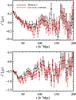 |
Fig. B.1
Comparison of the monopole and quadrupole correlation functions for the sample used here (black dots) and for the sample and continua of Lee et al. (2012b) (red dots). |
| Open with DEXTER | |
© ESO, 2013
Current usage metrics show cumulative count of Article Views (full-text article views including HTML views, PDF and ePub downloads, according to the available data) and Abstracts Views on Vision4Press platform.
Data correspond to usage on the plateform after 2015. The current usage metrics is available 48-96 hours after online publication and is updated daily on week days.
Initial download of the metrics may take a while.