| Issue |
A&A
Volume 550, February 2013
|
|
|---|---|---|
| Article Number | A4 | |
| Number of page(s) | 11 | |
| Section | Extragalactic astronomy | |
| DOI | https://doi.org/10.1051/0004-6361/201220355 | |
| Published online | 15 January 2013 | |
Online material
Appendix A: Study of the systematics
The systematic uncertainties on the EBL measurement with H.E.S.S. brightest blazars are investigated in this appendix. Following Sinervo (2003), two sources of systematics arising from “poorly understood features of the data or analysis technique” (class 2) and two sources of systematics arising “from uncertainties in the underlying theoretical paradigm” (class 3) are identified. The main class 2 systematic uncertainty is evaluated with Monte Carlo simulated air showers imaged by the detector and passing through the whole chain analysis (see, e.g., Aharonian et al. 2006a,and reference therein for a description of the Monte-Carlo simulations). The limited knowledge of the atmospheric conditions is accounted for with a toy model of the detector acceptance and distribution of events. Class 3 systematics are characterized in this study by the choice of template model for the EBL absorption and the selection of the best intrinsic model for each data set. The impact of the latter is evaluated with the data, testing ad hoc intrinsic models, while the former is compared with a concurrent modelling established by Domínguez et al. (2011).
A.1. Analysis chain
Monte Carlo data (see Aharonian et al. 2006a) were used to test the analysis chain. Four telescopes triggered events following a PWL of photon index 2 (hardest simulated index) were randomly removed from the simulated data set to create an artificial EBL attenuation. The data set studied was generated for a null azimuth and an off-axis angle of 0.5°. The zenith angle was fixed to 18°, close to the average zenith angle in the H.E.S.S. sky of PKS 2155 - 304, which is the source with the most important excess of γ-rays in this study (see Sect. 2.2). The EBL optical depth normalization α was then reconstructed with these samples of events following a spectrum φ(E) ∝ E-2exp( − α × τ(E,z)), where τ(E,z) is the FR08 EBL opacity and z the redshift of the source, fixed here to z = 0.1 for simplicity.
The background, particularly important for the spectral fit method described in Piron et al. (2001), was fixed to a tenth of the signal – comparable to the value derived for the first data set on PKS 2155 - 304. The reconstructed EBL normalization α is shown in the top panel of Fig. A.1 as a function of the simulated EBL normalization. The close match with the identity function strongly supports the reliability of the method employed.
The parameter that seems to affect the analysis chain the most is the background estimation, crucial for the mentioned spectral fit method. Imposing a background equivalent to a fiftieth of the signal, two samples of simulated events were studied for a null zenith and respective azimuths of 0° and 180°. The azimuth just indexes the data sets, since all azimuth angles are equivalent for a null zenith angle. The corresponding reconstructed EBL normalizations are represented with downward and upward triangles in the top panel of Fig. A.1. The associated error bars represent statistical uncertainties, related to the limited size of the Monte Carlo samples (typically 104 events), that must be taken into account when estimating the systematic uncertainty. A first (a priori naive) evaluation of this systematic is the average difference αreco − αsimu represented in the bottom panel, which reads 0.17 and 0.20 for each sample. A second evaluation is the maximum variation in the measurement Δ associated with a Gaussian statistic, yielding one standard deviation systematics Δ/ (see, e.g., Sinervo 2003) of 0.19 and 0.21, respectively. The estimate chosen is similar to the excess variance estimator developed by Vaughan et al. (2003) for variability. Assuming that the rms difference D between the simulated and reconstructed values is due to both statistical and systematic uncertainties, one would write
  , where
  is the variance estimator. We thus define the systematic uncertainty estimate as:
 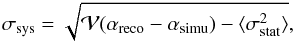 (A.1)which reads 0.15 and 0.26 for each sample. The global systematic error using both samples, σsys = 0.21, is shown in the top and bottom panels of Fig. A.1. This systematics estimate is similar to the two mentioned before, though a bit larger, which suggests a possible slight overestimation.
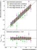 |
Fig. A.1
Reconstruction of the EBL normalization with Monte Carlo simulated air showers passing through the analysis chain. Three samples of Monte Carlo events are represented: the first one (orange squares) corresponds to the observation conditions of PKS 2155 - 304, the second and third (triangles) correspond to a poor background estimation. These two last sets were used to estimate the systematic uncertainty represented with the grey shaded area. Top panel: reconstructed EBL normalization as a function of the simulated normalization. Bottom panel: residuals, defined as the difference between the reconstructed and simulated optical depth normalizations. |
| Open with DEXTER | |
To ensure that a point-to-point systematic effect does not mimic the EBL absorption as a function of energy, a test was performed with a bright galactic source, the Crab Nebula, and yielded deviations to a null EBL normalization well below the systematic uncertainty derived for the analysis chain.
A.2. Choice of the intrinsic model
The second systematic uncertainty arises from the choice of the model for the intrinsic spectra. This systematic was assessed on the data by comparing the total likelihood profile derived with a LP for each intrinsic spectrum, on one hand, and with an EPWL, on the other. The corresponding likelihoods as a function of the EBL normalization are shown in Fig. A.2, where the maximum was set to unity for clarity. The comparison of third-order models such as ELP and SEPWL would only drown the systematic error in the statistical one. The two profiles were fitted with the procedure described in Sect. 3, yielding 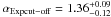 and
and  . Using the last systematic estimator described in the Sect. A.1, the difference between these two values due to the statistics is estimated to 0.14 (variance due to uncertainties), and the deviation caused by the systematics is 0.10.
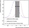 |
Fig. A.2
Likelihood profiles as a function of the normalized EBL opacity. The profiles were normalized to unity for clarity purposes. The dotted dashed curve is derived fitting log-parabolic intrinsic spectra to the data sets, while the dashed curve is derived by fitting exponential cut-off models. The gap between the two profiles due to the intrinsic spectral modelling is represented by the grey shaded area and the double arrow. |
| Open with DEXTER | |
To ensure the reliability of the measurement, three other selection criteria of the intrinsic model were tested. First, the model with the best χ2 probability was selected (as in the main method), but the flattest likelihood profile was used in case of ambiguity (e.g. between a LP and an EPWL), yielding a normalization of 1.18 ± 0.18, preferred at the 8.9σ level to a null opacity. A second approach consisted in choosing the simplest model, as long as the next order was not preferred at the 2σ level (taking the flattest profile in case of ambiguity), yielding a normalization of 1.46 ± 0.11, preferred at the 14.3σ level to a null opacity. These two criteria do not change the intrinsic model for the data sets on 1ES 0229+200, 1ES 1101-232, Mrk 421 (2), PKS 2005 - 489 (1 and 2), and PKS 2155 - 304 (1, 6, and 7). A final test consisted in imposing the most complex model (an ELP) on the other data sets, yielding a normalization of 1.29 ± 0.18, preferred at the 7.9σ level to a null opacity. The above-mentioned systematic uncertainty accounts for the slight changes induced by the selection method and the significance of the result remains almost unchanged.
It is worth noting that the particular attention paid to the intrinsic curvature of the spectra all along the analysis is not superfluous. The likelihood profile obtained assuming that the spectra are described by PWLs is maximum for αPowerLaw = 2.01 ± 0.07. The value derived with such a basic spectral model is significantly above the nominal normalized EBL opacity because intrinsic curvature of the spectra mimics the absorption effect.
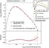 |
Fig. A.3
Toy-model of the energy distribution of H.E.S.S. events. The inset in the top panel shows the detector acceptance (black line) and the expected distributions of events for a PWL and an EBL absorbed PWL (green and brown lines, respectively). The injected spectra are shifted in energy to model the absorption of Cherenkov light by the atmosphere yielding the distribution of events shown in the top panel with brown filled circles. Fitting this distribution with a non shifted model enables the characterization of the atmospheric impact on the EBL normalization estimated to 0.05 for an energy shift of 10%. The residuals of the fit are shown in the bottom panel. |
| Open with DEXTER | |
A.3. Energy scale and choice of the EBL model
The atmosphere is the least understood component of an array of Cherenkov telescopes such as H.E.S.S. and can affect the absorption of the Cherenkov light emitted by the air showers. This absorption leads to a decrease in the number of photoelectrons and thus of the reconstructed energy of the primary γ-ray. The typical energy shift, of the order of 10% (Bernlohr 2000), does not affect the slope of a PWL spectrum, which is energy-scale invariant, but impacts its normalization. Indeed, for an initial spectrum φ(E) = φ0(E/E0) − Γ, an energy shift δ yields a measured spectrum  , where
  is the measured spectral normalization. Since the spectral analysis developed in this study relies on the EBL absorption feature which is not an energy-scale invariant spectral model, the atmosphere absorption impact on the measured EBL normalization is investigated.
A toy-model of the detector and of the atmosphere effect was developed to account for such a systematic effect. The detector acceptance  is parametrized as a function that tends to the nominal acceptance value at high energies, as in Eq. (A.2):
  (A.2)where is in m2, the energy E is in TeV, and a = 5.19, b = 2.32 × 10⁻², c = 3.14 are derived from the fit of the simulated acceptance. The number of events measured in an energy band dE is then simply
  , where the observation duration Tobs was fixed to impose a total number of events of 106. Typical event distributions for PWL and EBL absorbed PWL spectra are shown in the inset in Fig. A.3. A logarithmic energy binning of Δlog 10E = 0.1 is adopted and the uncertainty on the number of events in each energy bin is considered to be Poissonian. To model the effect of the atmosphere on the EBL normalization reconstruction, energy-shifted distributions
  were fitted with an non-shifted model, i.e.
  , with Eshift = (1 + δ) × E and φ(E) ∝ E − Γexp( − α × τ(E,z)). As mentioned above the effect on the index Γ is null because of the energy-scale invariance, which is not the case for the specific energy dependence of the EBL opacity. A toy-model distribution that was energy shifted is shown in the top panel of Fig. A.3 for a redshift z = 0.1 and an injected EBL normalization α = 1, corresponding to FR08 EBL modelling. The residuals Δlog 10(Nevents) to the fit of a non-shifted model are shown in the bottom panel.
The reconstructed and injected EBL normalizations differ by less than 0.05 for an energy shift of 10%, while the difference
can go up to 0.11 for an energy shift of 25%. The standard atmospheric conditions required by the data selection motivates the use of the 10% energy shift4 and thus leads to a systematic error due to Cherenkov light absorption of 0.05.
This toy model of the detector was also employed to compare independent EBL modellings. To probe a reasonable range of models, the lower and upper bounds on the EBL opacity derived by Domínguez et al. (2011) were used for the injected spectrum, while FR08 modelling was fitted to the event distribution. The variation in the reconstructed normalization is estimated to be 0.06 for a redshift z = 0.1. The small amplitude of the systematic effects of the atmosphere and of the EBL modelling choice (respectively 0.05 and 0.06) justifies a posteriori the use of the simple framework described in this section and does not motivate a deeper investigation.
© ESO, 2013
Current usage metrics show cumulative count of Article Views (full-text article views including HTML views, PDF and ePub downloads, according to the available data) and Abstracts Views on Vision4Press platform.
Data correspond to usage on the plateform after 2015. The current usage metrics is available 48-96 hours after online publication and is updated daily on week days.
Initial download of the metrics may take a while.