| Issue |
A&A
Volume 548, December 2012
|
|
|---|---|---|
| Article Number | A113 | |
| Number of page(s) | 24 | |
| Section | Interstellar and circumstellar matter | |
| DOI | https://doi.org/10.1051/0004-6361/201219792 | |
| Published online | 30 November 2012 | |
Online material
Appendix A: Previous images of the bow shock around Betelgeuse
For completeness, we show in this section the bow shock around Betelgeuse as observed with IRAS by Noriega-Crespo et al. (1997) (Fig. A.1) and AKARI by Ueta et al. (2008) (Fig. A.2).
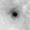 |
Fig. A.1
IRAS 60 μm image of the bow shock around Betelgeuse as detected by Noriega-Crespo et al. (1997). |
| Open with DEXTER | |
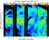 |
Fig. A.2
AKARI/FIS false-colour maps of α Ori in the SW bands – N60 (65 μm) and WIDE-S (90 μm) at 15′′/pixel scale – and in the LW bands – WIDE-L (140 μm) and N160 (160 μm) at 30′′/pixel scale – from left to right, respectively (Ueta et al. 2008). Background emission has been subtracted by a combination of temporal filters during data reduction. RA and Dec offsets (with respect to the stellar peak) are given in arcminutes. The wedges at the top indicate the log scale of surface brightness in MJy sr-1. North is up, and east to the left. |
| Open with DEXTER | |
Appendix B: Additional figures
Figure B.1 PACS 70 μm image on which concentric ellipses were fitted to the different arcs.
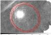 |
Fig. B.1
PACS 70 μm image overplotted in red with three concentric ellipses with the centre at α = 5h54m56.56s and δ = 7°22′16.18′′ radii of 622′′, 585′′, and 546′′ (as measured from the centre) and for a position angle of 47.7°. |
| Open with DEXTER | |
Appendix C: Herschel PACS image of R Leo
The Herschel PACS 70 μm image of the AGB star R Leo are compared to a hydrodynamical simulation in Fig. C.1. Rayleigh-Taylor instabilities, slightly deformed owing to the action of Kelvin-Helmholtz instabilities, are visible both in the data and in the simulations.
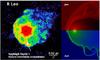 |
Fig. C.1
PACS 70 μm image of R Leo (left Cox et al. 2012) compared to a hydrodynamical simulation of the wind-ISM interaction computed with the AMRVAC code (van Marle et al. 2011). The parameters for this simulation are a stellar wind velocity of 15 km s-1, a constant gas mass-loss rate of 1 × 10⁻⁶ M⊙/yr, a dust-to-gas mass ratio of 0.01, a space velocity of 25 km s-1, a local ISM density of 2 cm-3, and an ISM temperature of 10 K. The upper right figure shows the gas density, which ranges (on log scale) between 10-24 and 10-19 g/cm3; the lower right figure represents the dust grain particle density, ranging (on log scale) between 10-10 and 10-3.5 cm-3. |
| Open with DEXTER | |
Appendix D: Dust grain temperature in the envelope around Betelgeuse
Under the assumption of a smooth continuous outflow and using the parameters as specified in Table 2, the dust grain temperatures for Fe and amorphous silicates in the envelope around Betelgeuse have been calculated using the mcmax code (Min et al. 2009). Only the stellar radiation is taken into account as the energy source to compute the dust temperatures assuming radiative equilibrium. The particle shape is represented by CDE (continuous distribution of ellipsoids Bohren & Huffman 1983) for particles of which the equivalent spherical grain would have a grain size of 0.1 μm. The composition of the amorphous silicates is taken from de Vries et al. (2010), who derived that the infrared spectrum of the AGB star Mira is best fitted with 65.7% MgFeSiO4 and 34.3% Mg2SiO4, implying an average composition of Mg1.36Fe0.64SiO4, having a β-index of ~1.8. The resulting dust temperatures are shown in Fig. D.1. The temperature for the amorphous silicate grains is lower than for the Fe-grains, owing to the higher opacity of Fe at the near-IR wavelengths, where the star emits most of its photons.
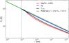 |
Fig. D.1
The dust-temperature profiles in the envelope of Betelgeuse as modeled with mcmax (Min et al. 2009). The different lines indicate the dust temperature of a specific dust species: red for amorphous silicates and blue for metallic iron. The full black line gives the mean dust temperature profile, assuming thermal contact between iron and amorphous silicate grains. The green lines show a power-law distribution for the dust temperature for β = 1. The vertical dashed line indicates the inner radius of the dust shell. |
| Open with DEXTER | |
Appendix E: Numerical simulations of the bow shock
E.1. Numerical method
For the simulations the MPI-AMRVAC hydrodynamics code (Keppens et al. 2012) was used. For a comparison to similar work, we refer to van Marle et al. (2011). The MPI-AMRVAC code solves the conservation equations for mass, momentum, and energy on an adaptive mesh grid. It includes optically thin radiative cooling, using the exact integration algorithm (Townsend 2009), and a cooling curve for gas at solar metallicity (Wang Ye, priv. comm.). For these simulations, a two-dimensional approach was taken, assuming an inclination angle of 0°. As deduced by Cox et al. (2012), the inclination angle of the space motion with respect to the plane of the sky is small (~8°).
Dust was included in the simulations using a two-fluid approach, where the dust is treated as a pressure-less fluid (Paardekooper & Mellema 2006; Woitke 2006a; van Marle et al. 2011; Cox et al. 2012). The dust is linked to the gas through the drag force (Kwok 1975): 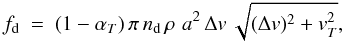 (E.1)with nd the dust particle density, ρ the gas density, a the radius of the dust grain,
  the thermal speed, and Δv the velocity difference between dust and gas. For a given mass, the particle density decreases with a-3. Therefore, the drag force is weaker for larger dust grains. The sticking coefficient for gas-dust collisions, αT, is estimated as
 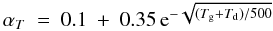 (E.2)(Decin et al. 2006), with Td the dust temperature and Tg the gas temperature. This is an improvement over our earlier simulations (van Marle et al. 2011; Cox et al. 2012), where we kept the sticking coefficient constant. Because the dust temperature is typically much lower than the gas temperature in the shocked CSM-ISM region, we approximate the sticking coefficient by setting Td = 08.
Unlike our previous models (van Marle et al. 2011; Cox et al. 2012), which used a cylindrical grid, these simulations are run on a two-dimensional spherical grid with a physical domain of R = 3 pc by θ = 180°. The grid has a minimal resolution of 160 radial by 80 azimuthal grid cells and five additional levels of refinement are allowed, giving the simulations an effective resolution of 2560 × 1280 grid cells.
E.2. Initial conditions
At the inner radial boundary, the wind parameters are set according to the values in Table 2. Since the star is moving relative to the ambient medium, the outer radial boundary is divided into two zones: (1) for θ < 90° an inflow boundary is set with the ambient gas entering the grid as a parallel stream with v = 28.3 km s-1; (2) for θ > 90° the gas is allowed to flow out of the grid. This is similar to the approach of Villaver et al. (2012). The gas density in the ambient medium is set at 3 × 10-24 g cm-3 (or nH ≈ 2 cm-3) and a temperature of 100 K (reflecting the temperature of a cold neutral medium). This temperature also serves as a lower limit for the gas temperature throughout the physical domain. We assume that there is no dust in the ambient medium.
To avoid numerical instabilities we start the simulation without radiative cooling and let it run for 100 000 years. By that time the bow shock has reached its equilibrium position (where the ram pressure of the wind is balanced by the ram pressure of motion of the star through the ambient medium). From this point in time we include radiative cooling and let the simulation run for 200 000 years.
Appendix F: Animations of bow shock simulations
Fig. F.1. Movie of Aori_TISM100K showing gas density and dust particle density for the 200 000 year period from the introduction of radiative cooling to the end of the simulation for the model with a cold ambient medium. (186.8 MB) (Access here)
Fig. F.2. Similar to Fig. F.1, Aori_TISM8000K showing the 200 000 year period from the introduction of radiative cooling to the end of the simulation for the model with a warm ambient medium. (188.9 MB) (Access here)
Fig. F.3. Similar to Fig. F.1, the third movie (Aori_vardM - ) shows the 200 000 year period from the introduction of radiative cooling to the end of the simulation for the model with a cold ambient medium and a varying mass-loss rate. (189.8 MB) (Access here)
Fig. F.4. Similar to Fig. F.2, the fourth movie (Aori_TISM8000K_highvel) shows the 200 000 year period from the introduction of radiative cooling to the end of the simulation for the model with a warm ambient medium and a high stellar velocity. (186.0 MB) (Access here)
Fig. F.5. Similar to Fig. F.1, the fifth movie (Aori_largegrain) shows the 200 000 year period from the introduction of radiative cooling to the end of the simulation for the model with a cool ambient medium, but for large (100 nm) dust grains. (189.8 MB) (Access here)
© ESO, 2012
Current usage metrics show cumulative count of Article Views (full-text article views including HTML views, PDF and ePub downloads, according to the available data) and Abstracts Views on Vision4Press platform.
Data correspond to usage on the plateform after 2015. The current usage metrics is available 48-96 hours after online publication and is updated daily on week days.
Initial download of the metrics may take a while.