| Issue |
A&A
Volume 546, October 2012
|
|
|---|---|---|
| Article Number | A43 | |
| Number of page(s) | 19 | |
| Section | Planets and planetary systems | |
| DOI | https://doi.org/10.1051/0004-6361/201219310 | |
| Published online | 05 October 2012 | |
Online material
Appendix A: Thermochemical data
Thermochemical properties, such as enthalpies of formation, entropies, and heat
capacities are very important to ensure the consistency between the rate parameters of
the forward and reverse elementary reactions. They are also useful for estimating the
heat release rate. Thermochemical data for all molecules or radicals have been estimated
and stored as 14 NASA polynomial coefficients, according to the McBride et al. (1993) formalism. The NASA polynomials take the
following form: 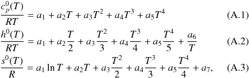 where
ai,
i ∈ [1,7] , are the numerical NASA coefficients
for the fourth-order polynomial. Each species is characterized by fourteen numbers. The
first seven numbers are for the high-temperature range, generally from 1000 to 5000 K,
and the following seven numbers are the coefficients for the low-temperature range,
generally from 300 to 1000 K. When these parameters are not available in the literature
(McBride et al. 1993) or in databases8, which is the most frequent case for species present
in automotive fuels, they have to be estimated. In this case, these data were
automatically calculated using the software THERGAS (Muller et al. 1995), which was developed in the LRGP laboratory and is based
on the group and bond additivity methods proposed by Benson (1976) and updated based on the data of Domalski & Hearing (1996). The enthalpies of formation of alkyl
radicals have been also updated according to the values of bond dissociation energies
published by Tsang & Hampson (1986) and
by Luo (2003) and following the recommendations
of Benson & Cohen (1997).
where
ai,
i ∈ [1,7] , are the numerical NASA coefficients
for the fourth-order polynomial. Each species is characterized by fourteen numbers. The
first seven numbers are for the high-temperature range, generally from 1000 to 5000 K,
and the following seven numbers are the coefficients for the low-temperature range,
generally from 300 to 1000 K. When these parameters are not available in the literature
(McBride et al. 1993) or in databases8, which is the most frequent case for species present
in automotive fuels, they have to be estimated. In this case, these data were
automatically calculated using the software THERGAS (Muller et al. 1995), which was developed in the LRGP laboratory and is based
on the group and bond additivity methods proposed by Benson (1976) and updated based on the data of Domalski & Hearing (1996). The enthalpies of formation of alkyl
radicals have been also updated according to the values of bond dissociation energies
published by Tsang & Hampson (1986) and
by Luo (2003) and following the recommendations
of Benson & Cohen (1997).
An elementary reversible reaction i involving L
chemical species can be represented in the general form
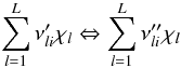 (A.4)where
 are the
forward stoichiometric coefficients, and
are the
forward stoichiometric coefficients, and  are the
reverse ones. χl is the chemical symbol of
the lth species.
are the
reverse ones. χl is the chemical symbol of
the lth species.
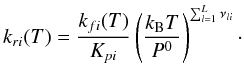
The kinetic data associated to each reaction are expressed with a modified Arrhenius
law 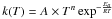 where T is the temperature, Ea the
activation energy of the reaction, A the pre-exponential factor, and
n a coefficient that allows the temperature dependence of the
pre-exponential factor. If the rate constant associated to the forward reaction is
kfi(T), then the one
associated to the reverse reaction is
kri(T), verifying
where T is the temperature, Ea the
activation energy of the reaction, A the pre-exponential factor, and
n a coefficient that allows the temperature dependence of the
pre-exponential factor. If the rate constant associated to the forward reaction is
kfi(T), then the one
associated to the reverse reaction is
kri(T), verifying
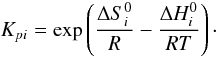
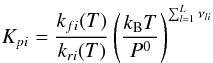 (A.5)where
Kpi is the equilibrium constant, when the
activity of the reactants is expressed in pressure units (Benson 1976):
(A.5)where
Kpi is the equilibrium constant, when the
activity of the reactants is expressed in pressure units (Benson 1976):
 (A.6)Here,
 and
and
 are the variation
in entropy and enthalpy occurring when passing from reactants to products in the
reaction i, P0 is the standard pressure
(P0 = 1.01325 bar), kB is the
Boltzmann’s constant, and νl are the
stoichiometric coefficients of the L species involved in reaction
i:
are the variation
in entropy and enthalpy occurring when passing from reactants to products in the
reaction i, P0 is the standard pressure
(P0 = 1.01325 bar), kB is the
Boltzmann’s constant, and νl are the
stoichiometric coefficients of the L species involved in reaction
i:  . Combined
with Eqs. (A.2) and (A.3),
. Combined
with Eqs. (A.2) and (A.3),
 and
and  can be calculated with the NASA coefficients:
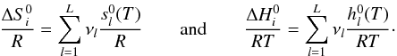 (A.7)Finally, we can
calculate the reverse reaction rate for the reaction i:
(A.7)Finally, we can
calculate the reverse reaction rate for the reaction i:
 (A.8)
(A.8)
Appendix B: Chemical equilibrium calculation
To compute the equilibrium abundance of the species in a definite system considered as
an ideal gas, we have developed a thermodynamical equilibrium calculator TECA. TECA is
software that allows equilibrium calculation for a complex mixture. More specifically,
for a given initial state of an ideal-gas mixture, the chemical-equilibrium program is
able to determine the gas composition at a defined temperature and pressure. This
calculation is based on the principle of the minimization of Gibbs energy (e.g. Gibbs 1873; White
et al. 1958; Eriksson & Rosen
1971; Smith & Missen 1982;
Reynolds 1986):
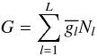 (B.1)where
L is the total number of species,
(B.1)where
L is the total number of species,
 the partial free energy of the species l, and
Nl the number of moles of the species
l.
the partial free energy of the species l, and
Nl the number of moles of the species
l.
The partial free energy of a compound l, behaving as an ideal gas, is
given by 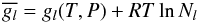 (B.2)where
gl(T,P) is the free
energy of the species l at the temperature T and the
pressure P of the system and R is the ideal gas
constant.
(B.2)where
gl(T,P) is the free
energy of the species l at the temperature T and the
pressure P of the system and R is the ideal gas
constant.
For an ideal gas, gl(T,P)
is given by 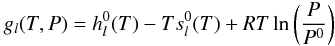 (B.3)where
 and
and
 are respectively, the
standard-state enthalpy and entropy of the species l at the temperature
T of the system.
are respectively, the
standard-state enthalpy and entropy of the species l at the temperature
T of the system.
The enthalpy and the entropy are expressed as NASA polynomials as described above.
Appendix C: Pressure-dependent reactions
Some examples of reactions with pressure-dependent rate constants present in the kinetic model.
Under some conditions, several reactions do not have the same rate constant depending on whether they occur under low or high pressure (respectively k0(T) and k∞(T)). In this case, between these two limits what is called a fall-off zone appears. This is typically the case in reactions requiring a collisional body to proceed, such as thermal dissociation or recombination (three-body) reactions. In the present kinetic model, we have different types of reactions with pressure-dependent rate constants (Table C.1). In some cases, some species act more efficiently as collisional bodies than do others. Then, when available from the literature, collisional efficiencies are used to specify the increased efficiency of the lth species in the ith reaction (see for example reaction (2) in Table C.1).
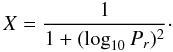
For the pressure-dependent reactions, the rate constant at any pressure is taken to be
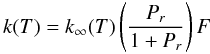 (C.1)where the reduced
pressure Pr is given by
(C.1)where the reduced
pressure Pr is given by
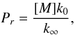 (C.2)and
[M] is the concentration of the mixture, weighted by the
efficiency of each compound, αl, in the
reaction studied:
(C.2)and
[M] is the concentration of the mixture, weighted by the
efficiency of each compound, αl, in the
reaction studied: 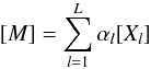 (C.3)where
[Xl] is the concentration of the
species k.
(C.3)where
[Xl] is the concentration of the
species k.
As shown in Table C.1, three methods of representation of the rate expression in the fall-off region are used (enhanced collisional body efficiencies of certain species are presented below the reaction):
-
the Lindemann et al. (1922)formulation, illustrated by reaction (1) inTable C.1;
-
the Troe (1983) formulation, see for example reaction (2) in Table C.1;
-
the SRI formulation proposed by Stewart et al. (1989), illustrated by reaction (3) in Table C.1.
In the Lindenman form, F is unity (F = 1).
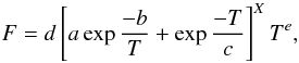
In the Troe form F is given by
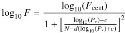 (C.4)with
 and
and
 (C.5)the
four parameters a, T***, T* and
T** must be specified but it is often the case that the parameter
T** is not used because of the lack of data.
(C.5)the
four parameters a, T***, T* and
T** must be specified but it is often the case that the parameter
T** is not used because of the lack of data.
The approach taken at the Stanford Research Institute (SRI) by Stewart et al. (1989) is in many ways similar to that taken by Troe,
but the blending function F is approximated differently. Here,
F is given by
 (C.6)where
 (C.7)
(C.7)
Appendix D: Photodissociations
Photodissociations scheme used in the model.
© ESO, 2012
Current usage metrics show cumulative count of Article Views (full-text article views including HTML views, PDF and ePub downloads, according to the available data) and Abstracts Views on Vision4Press platform.
Data correspond to usage on the plateform after 2015. The current usage metrics is available 48-96 hours after online publication and is updated daily on week days.
Initial download of the metrics may take a while.