| Issue |
A&A
Volume 544, August 2012
|
|
|---|---|---|
| Article Number | A76 | |
| Number of page(s) | 15 | |
| Section | Stellar structure and evolution | |
| DOI | https://doi.org/10.1051/0004-6361/201118352 | |
| Published online | 31 July 2012 | |
Online material
Appendix A: Equations
A.1. Determining parameters a, b, c and d (Eq. (2)) for the example of the LMC metallicity
In this section, we derive the parameters a, b, c and d of Eq. (2). This is done for the example of the LMC grid of stellar evolution models presented in Brott et al. (2011a).
Our dataset of the stellar evolution models contains information about the time-evolution of the surface nitrogen abundance. We can derive the main sequence lifetime from our models and therefore obtain the surface nitrogen abundance as a function of the fraction of the main sequence lifetime.
The parameter a corresponds to the initial surface nitrogen
abundance and is set to be the surface nitrogen abundance at τ = 0,
which for the LMC is given by the constant value  (A.1)By fitting
Eq. (2) to the data of the stellar
evolution models of the LMC grid, we obtain the remaining three parameters for
different masses and surface rotational velocities at the ZAMS.
(A.1)By fitting
Eq. (2) to the data of the stellar
evolution models of the LMC grid, we obtain the remaining three parameters for
different masses and surface rotational velocities at the ZAMS.
In Fig. A.1, the fitted parameter
b is shown as a function of vZAMS for
several different initial masses. A polynomial function of second order reproduces the
data for fixed mass well. The parameter b is therefore calculated as
 Figure A.2 shows the coefficients
b1, b2 and
b3 as a function of initial mass. They can be fitted
well by linear approximations shown by the solid lines. Using
b1(M),
b2(M) and
b3(M) the parameter
b(M [M⊙] ,vZAMS [km s-1] )
can be calculated using
Figure A.2 shows the coefficients
b1, b2 and
b3 as a function of initial mass. They can be fitted
well by linear approximations shown by the solid lines. Using
b1(M),
b2(M) and
b3(M) the parameter
b(M [M⊙] ,vZAMS [km s-1] )
can be calculated using  (A.2)Similarly we
obtained parameter c as a function of initial mass and surface
rotational velocity by fitting Eq. (2)
to the data of the stellar model grids. The result is shown in Fig. A.3 on the left panel. The data is fitted well as a
function of vZAMS using the polynomial function of second
order
(A.2)Similarly we
obtained parameter c as a function of initial mass and surface
rotational velocity by fitting Eq. (2)
to the data of the stellar model grids. The result is shown in Fig. A.3 on the left panel. The data is fitted well as a
function of vZAMS using the polynomial function of second
order  The
coefficients c1, c2 and
c3 are obtained for different initial masses to consider
a mass dependence.
The
coefficients c1, c2 and
c3 are obtained for different initial masses to consider
a mass dependence.
In the case of LMC models the dataset seen on the left panel in Fig. A.3 can be reproduced well by a linear function. Therefore parameter c1(M) is set to zero. This is not the case for SMC and MW were the polynomial function need to be used.
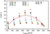 |
Fig. A.1
The parameter b is shown as a function of initial surface rotational velocity for several different masses, obtained by fitting Eq. (2) to the stellar evolution grid data (LMC). The solid line represents the best fit for the 30 M⊙ models. |
| Open with DEXTER | |
Figure A.3 shows the mass dependent
coefficients c2(M) and
c3(M) which can be fitted well using
linear functions shown by the solid lines. Using
c1(M),
c2(M) and
c3(M),
c(M [M⊙] ,vZAMS [km s-1] )
can be calculated by 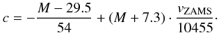 (A.3)Parameter
d is obtained for different masses and surface rotational
velocities at the ZAMS. The resulting values are shown in Fig. A.4. It can be seen, that only a weak mass dependence exists in the
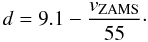
case of our data. For simplification, we neglect the mass dependence. Therefore a
linear approximation is used to describe parameter d as depicted in
Fig. A.4, which can be described by
(A.3)Parameter
d is obtained for different masses and surface rotational
velocities at the ZAMS. The resulting values are shown in Fig. A.4. It can be seen, that only a weak mass dependence exists in the
case of our data. For simplification, we neglect the mass dependence. Therefore a
linear approximation is used to describe parameter d as depicted in
Fig. A.4, which can be described by
 (A.4)
(A.4)
A.2. The main sequence lifetime and the surface rotational velocity
The fraction of the main sequence lifetime is used in Eq. (2) to calculate the surface nitrogen abundance. To be able to constrain the absolute age of the star it is necessary to know the time a star spends on the main sequence for given initial parameters.
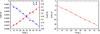 |
Fig. A.2
The three coefficients b1(M), b2(M) and b3(M) of the polynomial function to describe the parameter b are depicted as functions of mass. All parameters can be fitted well using linear functions which are plotted by solid lines. |
| Open with DEXTER | |
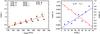 |
Fig. A.3
On the left panel, the parameter c is shown as a function of initial surface rotational velocity for several different masses. The line represents the best fit for the 30 M⊙ model. On the right panel, the coefficients c2(M) and c3(M) are plotted as functions of the initial mass. They can be reproduced best using linear functions shown by solid lines. |
| Open with DEXTER | |
We therefore derive a formula for the main sequence lifetime for stars of a given
initial mass and surface rotational velocity with MW, LMC and SMC metallicity.
Figure A.5 shows the main sequence lifetime as
a function of the initial surface rotational velocity for the example of the LMC data
for different initial masses. The higher the initial surface rotational velocity the
higher the main sequence lifetime. Considering Fig. A.5 it is noticeable that the main sequence lifetime is a strong function of
the initial mass, but shows only a weak dependence on the initial surface rotational
velocity. The data can be fitted well using 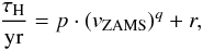 (A.5)taking mass
dependent parameters p,q and r into account. For
reproducing the data best, q is chosen to be a linear function of
mass, which in case of LMC and MW can be simplified to a constant value.
p and r can be calculated depending on the initial
mass. We therefore have
(A.5)taking mass
dependent parameters p,q and r into account. For
reproducing the data best, q is chosen to be a linear function of
mass, which in case of LMC and MW can be simplified to a constant value.
p and r can be calculated depending on the initial
mass. We therefore have 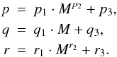 By
fitting the parameters p, q and r,
we gain the following formula to calculate the main sequence lifetime:
By
fitting the parameters p, q and r,
we gain the following formula to calculate the main sequence lifetime:
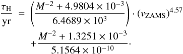 (A.6)In
our stellar evolution models, mass loss is included as described in Vink et al. (2010). During the main sequence
evolution the stars loses angular momentum due to mass loss. The value of the surface
rotational velocity therefore changes as a function of time. Figure A.6 depicts the surface rotational velocity of a few
exemplary models as functions of time (left panel) and effective temperature
Teff (right panel). An initial surface rotational
velocity of about 170 km s-1 is chosen.
(A.6)In
our stellar evolution models, mass loss is included as described in Vink et al. (2010). During the main sequence
evolution the stars loses angular momentum due to mass loss. The value of the surface
rotational velocity therefore changes as a function of time. Figure A.6 depicts the surface rotational velocity of a few
exemplary models as functions of time (left panel) and effective temperature
Teff (right panel). An initial surface rotational
velocity of about 170 km s-1 is chosen.
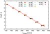 |
Fig. A.4
The parameter d is shown as a function of initial surface rotational velocity for several different masses, obtained by fitting Eq. (2) to the stellar evolution grid data (LMC). The line represents the best fit using a linear approximation. A small mass dependence can be seen, which will be neglected for simplification. |
| Open with DEXTER | |
During the evolution on the main sequence the surface rotational velocity of a star remains almost constant. At the end a sudden drop is visible for the highest considered masses, caused by an increase in mass loss and therefore a decrease of angular momentum when the effective temperature falls below 25 000 K, caused by the bi-stability braking (Vink et al. 2000, 2001). Stars with masses up to 30 M⊙ reach the end of the main sequence at temperatures higher than 20 000 K (see Fig. A.6). They do not stay long enough on the main sequence at Teff ≤ 25 000 K to be significantly slowed down. In the case of stars more massive than 30 M⊙ the assumption is valid for Teff ≥ 25 000 K. For stars which have not been influenced noticeably by this effect it is reasonable to estimate the surface rotational velocity by the value at the ZAMS.
A.3. Small Magellanic Cloud
For the SMC, the parameters specifying Eq. (2) are: 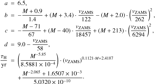
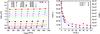 |
Fig. A.5
On the left panel the main sequence lifetime is shown as a function of the initial surface rotational velocity. Stellar evolution grid models for LMC metallicity are depicted for several different initial masses from 5 to 45 M⊙. The data can be fitted well using Eq. (A.5) as shown by the additional lines. On the right panel the two coefficients p and r are depicted as a function of mass. The dotted lines represent the best fit using Eq. (A.6). |
| Open with DEXTER | |
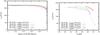 |
Fig. A.6
The evolution of the surface rotational velocity over time is shown on the left panel, while the surface rotational velocity as a function of the effective temperature is given on the right panel. Models of the stellar evolution grid in the case of LMC metallicity are used for different initial masses and surface rotational velocities of about 170 km s-1. |
| Open with DEXTER | |
The formula to calculate the main sequence lifetime for SMC stars is valid for all stars analyzed, but not in the complete range given in Table 2. Table A.1 summarizes the mass and velocity ranges valid for this specific formula.
Range of initial stellar parameters for which the main sequence lifetime calculation for SMC stars is validated.
A.4. Milky Way
For the MW, the parameters specifying Eq. (2) are: 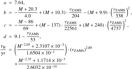
Appendix B: Dataset
Properties of the analyzed LMC stars.
Properties of the analyzed SMC stars.
© ESO, 2012
Current usage metrics show cumulative count of Article Views (full-text article views including HTML views, PDF and ePub downloads, according to the available data) and Abstracts Views on Vision4Press platform.
Data correspond to usage on the plateform after 2015. The current usage metrics is available 48-96 hours after online publication and is updated daily on week days.
Initial download of the metrics may take a while.