| Issue |
A&A
Volume 543, July 2012
|
|
|---|---|---|
| Article Number | A129 | |
| Number of page(s) | 17 | |
| Section | Extragalactic astronomy | |
| DOI | https://doi.org/10.1051/0004-6361/201219113 | |
| Published online | 10 July 2012 | |
Online material
Appendix A: Solving for the steady-state equations
 |
Fig. A.1
Computational domain in the (r,z) plane showing active and ghost grid zones with solid and dashed lines, respectively. The zone centers are marked with filled/open circles for active/ghost zones. The arrows indicate the backward finite-difference scheme used to discretize spatial derivatives. The innermost grid cell highlighted with a backslash palette refers to the seed value of the gas surface density n0,0. |
| Open with DEXTER | |
Figure A.1 shows the N × N computational mesh employed to discretize the steady-state Eqs. (3) and (4). The active zones are outlined with the solid lines, while the two rows of ghost zones (representing the reflecting boundary conditions along the z- and r-axes) are marked with the dashed lines. The active/ghost zone centers are denoted with filled/open circles.
A class of problems that does not require the knowledge of the gas density at the outer z and r boundaries (i.e., at N + 1 grid zones) can be solved using the following procedure. We use a first-order backward difference scheme (schematically shown by the arrows) to obtain a finite-difference representation of Eqs. (3) and (4) for the case with a spatially uniform σg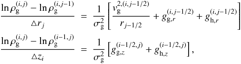 (A.1)where the indices i and j correspond to the z and r coordinate directions, respectively. We note that densities are defined at the zone centers while gravitational accelerations and velocities are defined at the corresponding zone interfaces. In order for this difference scheme to work, one needs to define the gas density at the ghost zones (which equal those at the nearest active zones) and also the gas density at the innermost active zone (1,1) denoted in the paper as the seed density n0,0. The corresponding zone is highlighted with the backslash palette in Fig. A.1.
With this choice of the discretization scheme and boundary conditions, one can notice that  and
and  are known for every value of
  and the latter can be found by a fast-forward substitution algorithm if one proceeds from left to right along the r-direction, starting from the bottom layer of zones and advancing one horizontal layer after another in the direction of increasing z.
Appendix B: Testing equilibrium configurations
An important reliability check on the solution procedure is to test how our equilibrium configurations can be handled by time-dependent numerical hydrodynamics codes. If our steady-state models are correct, a galaxy should stay in rotational equilibrium for at least 500 Myr, a typical time of interest when simulating the effect of supernova explosions in DGs.
To perform such a test, we used our time-dependent numerical hydrodynamics code employed earlier to study the effect of SN explosions in DGs in the local Universe and and high redshifts (Vorobyov et al. 2004; Vorobyov & Basu 2005; Vasiliev et al. 2008). We intentionally turned off cooling and heating to avoid the system drifting out of equilibrium due to thermal effects. For the test, we used the reference model with MDM = 109 M⊙, α = 0.9, Tg = 104 K, and n0,0 = 5.0 cm-3. The gas surface density, Q parameter, and velocity profiles of this model are shown by the red solid lines in the second top row of Fig. 2.
 |
Fig. B.1
Maximum and mean relative errors (dashed and solid lines, respectively) in the gas volume density (top) as functions of time t for the reference test model described in Appendix B. The errors are calculated relative to the initial equilibrium configuration at t = 0 Myr. The dash-dotted lines show the relative errors in the absence of gas self-gravity. |
| Open with DEXTER | |
Figure B.1 shows the mean relative error (solid line) and the maximum relative error (dashed line) in the gas volume density ρg (top) as a function of time t in our test model. The relative errors (in per cent) are calculated at every grid cell as12 (B.1)and demonstrate the degree to which our equilibrium is held by the code during the time evolution. The mean relative errors
  are calculated by averaging the individual errors △ ρg,i,j over the entire computational grid. As one can see, the mean relative errors never exceed 0.1%, meaning the equilibrium is well preserved globally. The maximum relative error never exceeds 3% and is kept below 1% during most of the evolution. We note the maximum errors occur in dynamically unimportant regions near the axes at large ϖ. The gas temperature shows essentially the same behavior. This test convincingly proves the robustness and reliability of our solution procedure.
To demonstrate the importance of gas self-gravity and to perform the final check on our self-gravitating equilibrium configurations, we artificially turned off the gas self-gravity in our time-dependent numerical hydrodynamics code. The dash-dotted lines in Fig. B.1 present the resulting mean relative error. Obviously, neglecting the gas self-gravity results in a complete destruction of the equilibrium state, with the mean relative errors exceeding 106 for the gas volume density!
© ESO, 2012
Current usage metrics show cumulative count of Article Views (full-text article views including HTML views, PDF and ePub downloads, according to the available data) and Abstracts Views on Vision4Press platform.
Data correspond to usage on the plateform after 2015. The current usage metrics is available 48-96 hours after online publication and is updated daily on week days.
Initial download of the metrics may take a while.