| Issue |
A&A
Volume 543, July 2012
|
|
|---|---|---|
| Article Number | A29 | |
| Number of page(s) | 27 | |
| Section | Stellar atmospheres | |
| DOI | https://doi.org/10.1051/0004-6361/201117222 | |
| Published online | 22 June 2012 | |
Online material
McDonald radial velocity measurements for HIP 56948.
Keck radial velocity measurements for HIP 56948.
Adopted atomic data, equivalent widths, and differential NLTE corrections (HIP 56948 – Sun).
Stellar parameters and Li abundance of HIP 56948 relative to the Sun (HIP 56948 – Sun).
Atomic and molecular line list in the vicinity of the Li lines.
Stellar abundances [X/H] in LTE and NLTE, and errors due to uncertainties in the stellar parameters.
Appendix A: Is the Tcond-abundance trend real?
We are just starting the era of high precision (0.01 dex) abundances studies, therefore the casual reader may question how real or universal is the abundance trend (⟨solar twins⟩ – Sun) with condensation temperature. The trend was first found by Meléndez et al. (2009), who determined a Spearman correlation coefficient of rS = +0.91 and a negligible probability of only ~10-9 of this trend to happen by pure chance. These results, based on Southern solar twins observed at the Magellan telescope, are reproduced in the left-upper panel of Fig. A.1, where the average abundance ratios of the solar twins is plotted against condensation temperature. Additional independent works are also shown in Fig. A.1, where a line representing the mean trend found by Meléndez et al. (2009), is superimposed upon the different samples.
The independent study by Ramírez et al. (2009), using McDonald data of Northern solar twins, follows the same trend (Fig. A.1, upper-right panel), as well as the average of six independent samples (Reddy et al. 2003; Allende Prieto et al. 2004; Takeda 2007; Neves et al. 2009; Gonzalez et al. 2010, Bensby et al., in prep.) of solar analogs in the literature (Ramírez et al. 2010), as shown in the left-middle panel of Fig. A.1.
The revision and extension (González Hernández et al. 2010) of the abundance analysis by Neves et al. (2009) of the HARPS high precision planet survey, also follows the same trend, except for a minor global shift of only − 0.004 dex, as illustrated in the right-middle panel of Fig. A.1. In this panel we show the average abundance ratios17 of 15 HARPS solar twins with Teff, log g and [Fe/H] within ± 100 K, ± 0.1 dex and ± 0.1 dex of the Sun’s stellar parameters. The agreement between the solar twin pattern of González Hernández et al. (2010) and the mean trend of Meléndez et al. (2009) is good, except for the element O and to a lesser extent for S, for which it is difficult to determine precise abundances. In particular, notice that González Hernández et al. (2010) derived oxygen abundances from the [OI] 630 nm line, which is badly blended with NiI. Also, notice that the [OI] feature is the weakest employed by them. Since their oxygen abundance is based on a single line, which is the weakest of all features analyzed by them, and that [OI] is blended with NiI, it is natural to expect that the O abundances in González Hernández et al. (2010) have the largest uncertainties. Furthermore, the HARPS spectra taken for planet hunting show some contamination from the calibration arc, so that abundances derived from only one single feature should be taken with care.
Regarding the analysis of individual stars, most of them also display the abundance trend, as shown for example for four solar twins in Fig. 2 of Ramírez et al. (2009) and 11 solar twins in Fig. 4 of Meléndez et al. (2009). Two new examples are shown in Fig. A.1. In the bottom-left panel we show the average abundance of the pair of solar analogs 16 Cyg A and B (Ramírez et al. 2011), based on high resolution (R = 60 000) and high S/N (~400) McDonald observations. As can be seen, this pair also follows the abundance trend, after a minor shift of −0.015 dex. In the bottom-right panel we show the abundance ratios of the solar twin 18 Sco (Meléndez et al. 2012, in prep.), based on high quality (R = 110 000, S/N ~ 800) UVES/VLT data. It is clear that the abundance trend is also followed by 18 Sco, after a shift of only +0.014 dex in the abundance ratios. Similar results are obtained using HIRES/Keck data (Meléndez et al. 2012, in prep.; see also Appendix B).
Thus, all recent high precision abundance studies based on different samples of solar twins and solar analogs in the Southern and Northern skies, using different instrumentation (Tull Coude Spectrograph at McDonald, MIKE at Magellan, HARPS at La Silla, UVES at the VLT, HIRES at Keck), show the abundance trend. In conclusion, it seems that the reality of the abundance trend found by Meléndez et al. (2009) and Ramírez et al. (2009), is well established.
 |
Fig. A.1
[X/Fe] ratios (from carbon to zinc) vs. condensation temperature for different samples of solar twins and solar analogs. The solid line represents the mean trend found by Meléndez et al. (2009). upper-left (filled circles): Southern sample of solar twins by Meléndez et al. (2009); upper-right (open circles): Northern solar twin sample by Ramírez et al. (2009); middle-left (squares): average of six different literature samples of solar analogs (Ramírez et al. 2010); middle-right (pentagons): average of 15 solar twins in the HARPS sample of González Hernández et al. (2010), after a shift of −0.004 dex; lower-left (triangles): average of the pair of solar analogs 16 Cyg A and B (Ramírez et al. 2011), after a shift of − 0.015 dex; lower-right (stars): abundance pattern of the solar twin 18 Sco (Meléndez et al. 2012, in prep.), after a shift of + 0.014 dex. |
| Open with DEXTER | |
Appendix B: Test of our precision using the asteroids Juno and Ceres
The referee suggested that we test our method using observations of two asteroids of different properties, obtained with the same instrument and setup, in order to show whether our very small standard errors (~0.005 dex) are adequate to estimate the observational uncertainties, as well as to look for potential systematic problems with the asteroid Ceres. Although we have not acquired such data yet, we do have observations of the solar twin 18 Sco and two different asteroids observed with different instruments: high quality UVES spectra of 18 Sco and the asteroid Juno (R = 110 000 and S/N ~ 800) and high quality HIRES spectra of 18 Sco and the asteroid Ceres (R = 100 000, S/N ~ 400). Juno is a S-type asteroid and Ceres is a C-type asteroid (e.g., DeMeo et al. 2009), therefore they have very different spectral properties and the relative analysis of 18 Sco to both Juno and Ceres should reveal if there is any problem in using their reflected solar light.
The analysis has been performed as described in Sect. 3. Our preliminary LTE results for the stellar parameters of 18 Sco are Teff = 5831 ± 10 K, log g = 4.46 ± 0.02 dex, [Fe/H] = 0.06 ± 0.01 dex. Full details of the abundance analysis will be published elsewhere. In Fig. B.1 we show the difference between the [X/H] ratios obtained in 18 Sco using the Ceres and Juno asteroids, [X/H]18Sco−Ceres – [X/H]18Sco−Juno, or in other words the abundance difference (Juno – Ceres). Notice that the same set of lines was used for both analyses. The error bars shown in Fig. B.1 are the combined error bar based on the standard error (s.e.) of each analysis, i.e., error =  .
.
As can be seen, the standard errors fully explain the small deviations of the (Juno–Ceres) abundance ratios. The mean difference ⟨Juno – Ceres⟩ is only 0.0017 dex, and the element-to-element scatter is only 0.0052 dex, meaning that each of the individual analyses should have typical errors of about 0.003–0.004 dex. The agreement is very satisfactory considering the different instrumentation employed and that the comparison between Juno and Ceres is done through a third object (the solar twin 18 Sco). Also, notice that there is no meaningful trend with condensation temperature. The test performed here strongly supports for our high precision and removes the possibility that the abundance trend may arise due to the particular properties of asteroids.
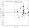 |
Fig. B.1
Differences between the solar abundances obtained with the asteroids Juno and Ceres, obtained from (Juno – Ceres) = [X/H] (18 Sco – Ceres) – [X/H](18 Sco – Juno). The solid line shows the mean difference and the dotted lines show the element-to-element scatter. |
| Open with DEXTER | |
Besides the potential applications of high precision differential abundance techniques to study the star-planet connection, these techniques are also giving new insights in other areas. Nissen & Schuster (2010) achieved uncertainties of 0.03 dex in [Mg/Fe] and only 0.02 dex in both [Ca/Fe] and [Ti/Fe], showing a clear separation of the halo into two distinct populations with different [α/Fe] ratios. Regarding globular clusters, Meléndez & Cohen (2009) have shown that CN-weak giants in M71 show a star-to-star scatter in [O/Fe] and [Ni/Fe] of only 0.018 dex, while [Mg/Fe] and [La/Fe] have a scatter of 0.015 dex. The star-to-star scatter in metallicity ([Fe/H]) is only 0.025 dex. Even a lower star-to-star scatter is found among “globular cluster star twins” (stars within ± 100 K of a globular cluster standard star) of NGC 6752. Using superb spectra (R = 110 000; S/N = 500) obtained with UVES on the VLT (Yong et al. 2003, 2005) and applying similar techniques to those presented in Sect. 3, Yong et al. (in prep.) have found an unprecedentedly low star-to-star scatter of only 0.003 dex in the iron abundances among NGC 6752 star twins, revealing chemical homogeneity in this cluster at the 0.7% level.
Appendix C: Determination of stellar parameters
As mentioned in Sect. 3, the excitation and ionization equilibrium do not depend only on Teff and log g, respectively. There is some dependence with other stellar parameters, but to a much lesser extent, such that a “unique” solution can easily be obtained after a few iterations. In practice, considering the weak degeneracies, a first guess of the effective temperature can be obtained by computing the slope at three different Teff (e.g., in steps of 50 K and at fixed solar log g) at the best microturbulence velocity (at a given Teff and log g). Then a linear fit is performed to Teff vs. slope (see Fig. C.1) to find the effective temperature at slope = 0. Then, for this Teff we can run three models with different log g (e.g., in steps of 0.05 dex in log g) in order to find the best surface gravity, by fitting log g vs. ΔII − I (see Fig. C.2), and for each model the microturbulence is obtained. This leads to the first guess of Teff, log g and vt. Further iterations at smaller steps (down to 1 K in Teff, 0.01 dex in log g and 0.01 km s-1 in vt) can quickly lead to the best solution that simultaneously satisfies the conditions of differential spectroscopic equilibrium (Eqs. (2)–(4)).
In Fig. C.1 we show that the excitation equilibrium provides a precise Teff. In this figure, effective temperature is plotted versus the slope =  . As can be seen, there is a clear linear relation between Teff and the slope, with some minor spread of only 0.8 K due to a range in adopted surface gravities.
 |
Fig. C.1
Teff as a function of the slope = |
| Open with DEXTER | |
Regarding the ionization equilibrium, we show in Fig. C.2 the dependence between surface gravity and ΔII − I (see Eq. (3)). A linear fit represents this relation well, with a scatter in log g of only 0.006 dex for models in a range of effective temperatures.
 |
Fig. C.2
Surface gravity vs. ΔII − I = (3ΔFeII − FeI + 2ΔTiII − TiI + ΔCrII − CrI)/6 (see Eq. (3)). The spread of the circles corresponds to a range of effective temperatures (5791 K ≤ Teff ≤ 5797 K), implying a scatter of 0.006 dex in log g. The line represents a linear fit. |
| Open with DEXTER | |
In Fig. C.3 we show the linear dependence between microturbulence velocity and the slope  . For a given model, vt could be constrained to within 0.0004 km s-1. A range in Teff (5791 K ≤ Teff ≤ 5797 K) and log g (4.40 dex ≤ log g ≤ 4.52 dex) imply in a scatter of only 0.009 km s-1 in vt.
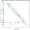 |
Fig. C.3
Microturbulence velocity vs. slope |
| Open with DEXTER | |
Given the above dependences, the stellar parameters Teff, log g and vt must be iteratively modified until the spectroscopic equilibrium conditions (Eqs. (2)–(4)) are satisfied simultaneously. Since the degeneracy is relatively small, the final solution (Teff/log g/vt = 5794 K/4.46 dex/1.00 km s-1) is very close to the independent solutions shown in Figs. C.1–C.3 (5794.5 K/4.458 dex/1.006 km s-1).
In order to check how unique the derived final solution is, we have run over 200 models with different stellar parameters, with a very fine grid (steps of only 1 K in Teff and 0.01 dex in log g) near our best solution. We then evaluated how close to zero are the slope in Teff (Eq. (2)) and the ionization equilibrium parameter ΔII−II (Eq. (3)). The following quantity is evaluated for each model,  (C.1)The model showing the lowest TG value would be the best spectroscopic solution, which in our case is obtained for Teff = 5794 K, log g = 4.46 dex, and vt = 1.00 km s-1. A contour plot for the TG parameter is shown in Fig. C.4. Besides the best solution at Teff = 5794 K and log g = 4.46 dex, there are a few other nearby plausible solutions, with a mean value at Teff = 5794.3 ± 0.5 K and log g = 4.462 ± 0.012 dex, shown by a cross in Fig. C.4. Our grid samples a much larger coverage than that shown in Fig. C.4, and we have verified that the best solution indeed represents a global minimum, i.e., there is no other solution that can simultaneously satisfy the conditions of differential spectroscopic equilibrium. Thus, within the error bars our solution is “unique”.
 |
Fig. C.4
Contour plot of the parameter TG (Eq. (C.1)), which evaluates how good the differential spectroscopic equilibrium is. The minimum is shown by a cross at Teff = 5794.3 ± 0.5 K and log g = 4.462 ± 0.012 dex, which is in excellent agreement with our adopted solution. The contour levels increase in steps of ΔTG = 0.1 from the minimum. |
| Open with DEXTER | |
Appendix D: Helium abundance and the age and log g of HIP 56948
Since our stellar parameters are very precise, the He abundance in HIP 56948 actually cannot be arbitrarily different from the solar He abundance. For example, an evolutionary track computed with a He abundance 5% higher than solar, would shift the Teff by about +74 K at the same log g, i.e., a change 10 times larger than our error bar in Teff, thus leading to no plausible solutions. We are currently building an extensive grid of models with He as a free parameter, using the Dartmouth stellar evolution code (Chaboyer et al. 2001; Guenther et al. 1992), which is based upon the Yale stellar evolution code.
In Fig. D.1, we show evolutionary tracks for M = 1.012 M⊙ (solid lines), which is the best mass found for HIP 56948 using the Dartmouth tracks, adopting the He solar abundance. These models were computed at three different helium abundances, solar and ± 1% solar. We also show isochrones at 3 and 4 Gyr for different He abundances. The error bars in log g and Teff put constraints on the He abundance, which can not be radically different from solar. Notice that the isochrones run parallel to each other and with only a minor shift for a change of ± 1% in the He abundance, thus resulting in about the same central solution for age, independent of the adopted He content. Therefore thanks to our small error bars in stellar parameters we can put stringent constraints on the age of HIP 56948. Interestingly, there is a degeneracy between He and mass, although below our 2% error bar in mass.
Another example where the adoption of a somewhat different He abundance did not affect the stellar age much is for the pair of solar analogs 16 Cyg A and B. For this pair, asteroseismology have recently constrained the ages of these stars, which are in excellent agreement with those derived from our isochrone technique, despite the somewhat different adopted He abundances. Based on three months of almost uninterrupted Kepler observations, Metcalfe et al. (2012) obtained an age = 6.8 ± 0.4 Gyr for their optimal models, in excellent agreement with an age = 7.1 ± 0.4 Gyr derived from our isochrone technique for the 16 Cyg pair (Ramírez et al. 2011).
 |
Fig. D.1
Solar metallicity evolutionary tracks for 1.012 M⊙ (solid lines) at three different He abundances: solar and ± 1% solar. Isochrones at 3 and 4 Gyr are plotted with dashed lines. The position of HIP 56948 and error bars in Teff and log g are also shown. |
| Open with DEXTER | |
The effect of changing He by ± 1% (in Y) in our model atmospheres has also a minor impact on the derived spectroscopic log g. As shown by Stromgren et al. (1982), for solar type dwarfs
the change in log g due to a change in the helium to hydrogen ratio (y = NHe/NH) is: 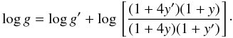 (D.1)Lind et al. (2011b) have shown that the relation above is also adequate for giant stars. For a change of +1% in Y in HIP 56948, the predicted change in log g is only − 0.001 dex, which is well below our error bar in log g (0.02 dex). Thus, assuming that the He abundance of HIP 56948 is not radically different from solar, our derived spectroscopic log g value is essentially unaffected.
Appendix E: v sin i and macroturbulence velocity
We have determined v sin i from the differential line broadening (HIP 56948 – Sun). Naively we could be assuming an identical macroturbulence for both stars, but at a given luminosity class, macroturbulence seems a smooth function of temperature (e.g., Saar & Osten 1997; Gray 2005; Valenti & Fischer 2005), so neglecting this effect can lead to a slight overestimation of v sin i in HIP 56948 because it is hotter than the Sun and therefore the contribution of vmacro to the line broadening in HIP 56948 should be slightly larger.
The trend of macroturbulence velocity with Teff described by Gray (2005) for main sequence stars18 can be fitted by  (E.1)A similar correlation was advocated by Valenti & Fischer (2005) (after normalization to
  = 3.50 km s-1, which is the value obtained for the Sun using Gray’s relation):
  (E.2)Finally, the mean relation (active and non-active stars) obtained by Saar & Osten (1997), after transforming (B − V) to Teff (Valenti & Fischer 2005) and normalizing it to
  km s-1, is:
  (E.3)The first two relations are valid for ~5000–6500 K, while the last relation is valid for ~5000–6100 K. On average, the above relations predict a differential (HIP 56948 – Sun) Δvmacro = 0.044 ± 0.018 km s-1.
In order to determine v sin i we selected 19 lines in the 602 − 682 nm region, although essentially similar results are obtained (albeit with ever so slightly larger errors) when 50 lines covering the 446–682 nm region are used. First, we performed spectral synthesis of selected lines, in order to calibrate the relation between line width (in Å) and total broadening (in km s-1). Then, we estimated the total broadening using a much larger set of lines, and obtained v sin i after subtracting both the instrumental and the macroturbulence broadening.
After taking into account the somewhat higher macroturbulence velocity of HIP 56948, we find v sin i/vsini⊙ = 1.006 ± 0.014, or Δ v sini = + 0.013 ± 0.026 km s-1 (or ± 0.032 km s-1 including the error in macroturbulence), i.e., HIP 56948 seems to have about the same rotation velocity as the Sun, or rotating slightly faster, although it is unclear how much faster due to the uncertain sin i factor.
© ESO, 2012
Current usage metrics show cumulative count of Article Views (full-text article views including HTML views, PDF and ePub downloads, according to the available data) and Abstracts Views on Vision4Press platform.
Data correspond to usage on the plateform after 2015. The current usage metrics is available 48-96 hours after online publication and is updated daily on week days.
Initial download of the metrics may take a while.