| Issue |
A&A
Volume 542, June 2012
GREAT: early science results
|
|
|---|---|---|
| Article Number | L19 | |
| Number of page(s) | 6 | |
| Section | Letters | |
| DOI | https://doi.org/10.1051/0004-6361/201218907 | |
| Published online | 10 May 2012 | |
Online material
Appendix A: The APEX observations
Observed lines and corresponding telescope parameters for the APEX observations of W28F.
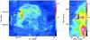 |
Fig. A.1
Location of the field covered by our CO observations on the larger-scale radio continuum image at 327 MHz taken from Claussen et al. (1997): entire SNR in the left panel, zoom in the right panel. The shown CO observations are the (6–5) map, also displayed in Fig. 1. |
| Open with DEXTER | |
APEX observations towards the supernova remnant W28F were conducted in several runs in the year 2009 (in May, June, August and October). We used of a great part of the suite of heterodyne receivers available for this facility: APEX–2 Risacher et al. (2006), FLASH460 Heyminck et al. (2006), and CHAMP+Kasemann et al. (2006); Güsten et al. (2008), in combination with the MPIfR fast Fourier transform spectrometer backend (FFTS, Klein et al. 2006). The central position of all observations was set to be 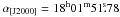 , β[J2000] = −23°18′58
 50. Focus was checked at the beginning of each observing session, after sunrise and/or sunset on Mars, or on Jupiter. Line and continuum pointing was locally checked on RAFGL1922, G10.47B1, NGC 6334-I or SgrB2(N). The pointing accuracy was found to be of the order of 5″ rms, regardless of the receiver that was used. Table A.1 contains the main characteristics of the observed lines and corresponding observing set-ups: frequency, beam size, sampling, used receiver, observing days, forward and beam efficiency, system temperature, spectral resolution, and finally the velocity interval that was used to generate the integrated intensity maps. The observations were performed in position-switching/raster mode using the APECS software Muders et al. (2006). The data were reduced with the CLASS software (see http://www.iram.fr/IRAMFR/GILDAS). For all observations, the maximum number of channels available in the backend was used (8192), except for CO (4–3), for which only 2048 channels were used, leading to the spectral resolutions indicated in Table A.1. Maps were obtained for all considered transitions, covering the field introduced in Fig. 1 and put in the perspective of the whole SNR in Fig. A.1.
Appendix B: The H2 observations
B.1. The dataset
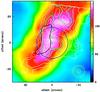 |
Fig. B.1
Overlay of the map of CO (6–5) emission observed by the APEX telescope (colour background) with the H2 0–0 S(5) emission (white contours), observed with the Spitzer telescope. The wedge unit is K km s-1 (antenna temperature) and refers to the CO observations. The H2 0–0 S(5) contours are from 50 to 210σ, in steps of 20σ ≃ 1.6 × 10⁻⁴ erg cm-2 s-1 sr-1. The green contour defines the half-maximum contour of this transition. Like in Fig. 1, the blue circle indicates the beam size of the SOFIA/GREAT observations, on the position of the centre of the circle, marked by a blue dot. The beam and pixel sizes of the CO (6–5), and H2 0–0 S(5) observations are also provided in yellow (big and small, respectively) circles in the lower right corner. The black contour delineates the half-maximum contour of the H2 0–0 S(2) transition. The field is smaller than in Fig. 1, and the (0, 0) position is that of the Spitzer observations (see Appendix B). |
| Open with DEXTER | |
As a consistency check for our models, we used of the Spitzer/IRS observations of the H2 pure rotational transitions (0–0 S(0) up to S(7)), reported and analysed in N07 and Y11. Although the original dataset also includes other ionised species, we chose to use only the H2 data. The raw product communicated to us by David Neufeld contains rotational transitions maps, with 1.2″ per pixel, centred on 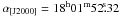 , β[J2000] = −23°19′2492. Figure B.1 shows an overlay of our APEX CO (6–5) map with the H2 0–0 S(5) region observed by Spitzer. The figure shows coinciding maxima between the two datasets in the selected position, and a slightly different emission distribution. This might be the effect of the better spatial resolution of the H2 data, which reveal more peaks than in CO. This overlay also shows the slightly different morphology of the emission of the S(2) (half maximum contour in black) and S(5) (half maximum contour in green) transitions, at the available resolution.
B.2. Excitation diagram
We performed a consistency check on our modelling (see Sect. 3) using the excitation diagram derived for the selected emission region. The H2 excitation diagram displays ln(Nνj/gj) as a function of Eνj/kB, where Nνj (cm-2) is the column density of the rovibrational level (v,J), Eνj/kB is its excitation energy (in K), and gj = (2j + 1)(2I + 1) its statistical weight (with I = 1 and I = 0 in the respective cases of ortho- and para-H2). If the gas is thermalised at a single temperature, all points in the diagram fall on a straight line. The selected position for the present study was introduced in Sect. 2.1, and can be seen in Figs. 1 and B.1. The column density of the higher level of each considered transition was extracted by averaging the line intensities in a 11.85″ radius circular region, consistent with our handling of the CO data. In the process, we corrected the line intensities for extinction, adopting the visual extinction values from N07, Aν = 3 − 4, and using the interstellar extinction law of Rieke & Lebofsky (1985). The resulting excitation diagram can be seen in Fig. B.2. We note that the intensity of the H2 0–0 S(6) transition (J = 8) cannot be determined reliably, because the line is blended with a strong 6.2 μm PAH feature.
B.3. Comparisons with our models
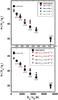 |
Fig. B.2
H2 excitation diagram comparisons. Upper panel: evolution of the modelled excitation diagram obtained for ζ1 = 5 × 10-17 s-1, varying the initial value of the OPR from the unrealistic, extreme-case 0 value to its equilibrium one, 3. Lower panel: influence of the cosmic ray ionisation rate variation on our modelled excitation diagram, with the initial OPR set to 3. |
| Open with DEXTER | |
Unlike our CO observations, the Spitzer/IRS observations are not spectrally resolved (owing to the relatively low resolving power of the short low module, in the range 60–130). On the other hand, given the minimum energy of the levels excited in the H2 transitions (for 0–0 S(0), Eu ~ 509.9 K), we can make the double assumption that the lines are not contaminated by ambient emission or self-absorption, and that the measured line intensities are the result from the blue- and red-shock present in the line of sight. Therefore, one must compare the observed H2 level populations to what is generated by the sum of our best-fitting blue- and red-shock models. Figure B.2 shows the comparison between the excitation diagram derived from the sum of our two CO best-fitting models and the observed one. The H2 excitation diagram comprising the sum of our CO best-fitting models is shown in both panels in red circles, and provides a satisfying fit to the observations. With the aim of improving the quality of this fit, we also studied the influence of the initial ortho-to-para ratio (OPR) value, upper panel, and of the cosmic ray ionisation rate value, lower panel.
In the upper panel, for a cosmic ray ionisation rate value adopted as the solar one, ζ1 = 5 × 10-17 s-1, the influence of the initial OPR value is studied. In their models, N07 inferred a value of 0.93 for the “warm” component (~322 K). On the other hand, the value associated to their “hot” (~1040 K) component could not be estimated, owing to the large uncertainty associated to the determination of the H2 0–0 S(6) flux. In our shock models, the OPR value is consistently calculated at each point of the shocked layer, and is mostly the result of conversion reactions between H2 and H, H+ or H . The heating associated to the passage of the wave increases the OPR value towards the equilibrium value of 3.0. Nevertheless, this value is reached only when it is also the initial one. The N07 situation is then probably adequately approximated in our models where the OPR initial value is less than 3. However, the influence of this parameter is minimal on the excitation diagram, where it only seems to create a slight saw-tooth pattern between the odd and even values of J.
We finally investigated the effects of the high-energy radiation field on the excitation diagram in the lower panel of Fig. B.2. The limits of our modelling are reached because the only handle that we have to study this effect on our outputs is the variation of the cosmic ray ionisation rate value, which affects the corresponding chemistry (higher ionisation fraction) and physics (warmer gas). A proper treatment of the energetic radiation components listed in Hewitt et al. (2009) should indeed incorporate UV pumping or self-shielding, as would be the case in PDR regions (e.g., Habart et al. 2011), as well as chemical and H2 excitation effects by X-ray (see Dalgarno et al. 1999) and cosmic rays (e.g., Ferland et al. 2008). Keeping these limits in mind, we found that even strong modifications of the cosmic ray ionisation rate from the solar value of 5 × 10-17 s-1 to the more extreme value of 10-14 s-1 have only very limited effects on the excitation diagram. The rather convincing fits to the H2 data seem to indicate that these excitation effects by energetic photons could well be minimal in our case, but we repeat that their proper inclusion to our models is work in progress.
© ESO, 2012
Current usage metrics show cumulative count of Article Views (full-text article views including HTML views, PDF and ePub downloads, according to the available data) and Abstracts Views on Vision4Press platform.
Data correspond to usage on the plateform after 2015. The current usage metrics is available 48-96 hours after online publication and is updated daily on week days.
Initial download of the metrics may take a while.