| Issue |
A&A
Volume 540, April 2012
|
|
|---|---|---|
| Article Number | A71 | |
| Number of page(s) | 16 | |
| Section | Planets and planetary systems | |
| DOI | https://doi.org/10.1051/0004-6361/201117687 | |
| Published online | 28 March 2012 | |
Online material
Appendix A: Additional figures
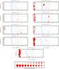 |
Fig. A.1
End-states (in 5 Myr) of the simulations starting with 28 embryos, each with 3 M⊕. The simulations are separated by horizontal dashed green lines. The surviving embryos/cores are shown with filled red dots, whose size is proportional to the objects’ mass. The scale is shown in the bottom panel. The red horizontal bar shows the perihelion-aphelion excursion of these objects on their eccentric orbits. The objects beyond 15 AU are plotted for simplicity at 15.5 AU, beyond the vertical solid green line. Jupiter and Saturn are shown as blue asterisks. The label on top of each panel reports the number N of embryos and the values of fI and fd adopted in the simulations. (For the discussion – see Sect. 4.) |
| Open with DEXTER | |
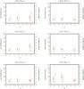 |
Fig. A.2
Statistical analysis of the results of the simulations starting from 28 embryos, each with 3 M⊕. The x-axis of left plots reports the value of fI at fixed fd, given at the title of each plot. Similarly, the x-axis of right plots reports the value of fd at fixed fI. The dot, slightly displaced to the left, is the mean mass of the largest core surviving beyond Saturn, computed over the corresponding ten simulations. The thick vertical bar is the rms deviation of this quantity. The thin bar shows the excursion of the same quantity from minimum to maximum. The square in the middle and related bars are the same, but for the second-largest core. The mass scale is reported left of the diagram. The cross, slightly displaced to the right, reports the mean number of embryos/cores surviving beyond Saturn, to be read against the scale on the right hand side. Again, the thick bar is for the rms deviation and the thin bar for the minimum-maximum quantity. (For the discussion – see Sect. 4.) |
| Open with DEXTER | |
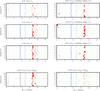 |
Fig. A.3
Same as Fig. A.1 but for the simulations in which the planet trap was considered. The plots a)–c) show the end-states starting with initial embryo-mass of 3 M⊕ when the turbulence is not taken into account, plots d)–f) are related to the cases with the turbulence characterized by γ = 3 × 10⁻⁴, 1 × 10⁻³, and 3 × 10⁻³, respectively. At the start, ten embryos are assumed in these simulations. Plot g) shows the end-states of simulations starting with a higher total mass (15 embryos of 3 M⊕) and plot h) does this for a larger number of initally less massive embryos (30 embryos of 1 M⊕). (For the discussion – see Sect. 5.) |
| Open with DEXTER | |
 |
Fig. A.4
Same as Fig. A.3 but with the initial mass of each embryo of 1.5 M ⊕ . (For the discussion – see Sect. 6.1.) |
| Open with DEXTER | |
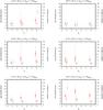 |
Fig. A.5
Same as Fig. A.2 but with the initial mass of each embryo of 1.5 M⊕. (For the discussion – see Sect. 6.1.) |
| Open with DEXTER | |
© ESO, 2012
Current usage metrics show cumulative count of Article Views (full-text article views including HTML views, PDF and ePub downloads, according to the available data) and Abstracts Views on Vision4Press platform.
Data correspond to usage on the plateform after 2015. The current usage metrics is available 48-96 hours after online publication and is updated daily on week days.
Initial download of the metrics may take a while.