| Issue |
A&A
Volume 539, March 2012
|
|
|---|---|---|
| Article Number | A65 | |
| Number of page(s) | 19 | |
| Section | Galactic structure, stellar clusters and populations | |
| DOI | https://doi.org/10.1051/0004-6361/201117977 | |
| Published online | 24 February 2012 | |
Online material
Appendix A: The dynamical models
A.1. Spherical isotropic King models
The King (1966) one-component, spherical, isotropic models are based on the following distribution function: 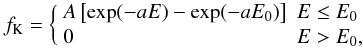 (A.1)
(A.1)
where A, a, E0 are positive constants, defining two scales and one dimensionless parameter, and E represents the specific energy E = v2/2 + Φ(r), where Φ(r) is the mean-field gravitational potential, to be determined from the Poisson equation. The quantity E0 is a threshold energy, above which the stars are considered unbound; it can be translated into a truncation radius, rtr, for the system.
We recall that the radial scale r0 can be defined as 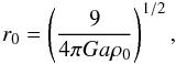 (A.2)where ρ0 is the central mass density. The other dimensional scale is the total mass of the cluster or, as an alternative, its central velocity dispersion.
The dimensionless concentration parameter is given by the central dimensionless potential Ψ = a [Φ(rtr) − Φ(0)] or, alternatively, by the index  (A.3)because these two quantities are in a one-to-one relation.
The quantity listed in the Harris catalog as concentration parameter, in this paper indicated with C, is defined using the standard core radius Rc in place of r0 in Eq. (A.3). The values of C for a model identified by Ψ ≳ 4 are slightly larger than the corresponding values of c; in fact, for these models 0.8 ≲ Rc/r0 ≲ 1.
A.2. Anisotropic f(ν) models
Several families of dynamical models have been developed to represent the final state of numerical simulations of the violent relaxation process thought to be associated with the formation of bright elliptical galaxies via collisionless collapse (for a review, see Bertin & Stiavelli 1993). These models show a characteristic anisotropy profile, with an inner isotropic core and an outer envelope that becomes dominated by radially-biased anisotropic pressure. They provide a good representation of the photometric and kinematic properties of elliptical galaxies. Here we will refer to the family of spherical, anisotropic, non-truncated f(ν) models (which have been revisited recently in detail by Bertin & Trenti 2003).
The distribution function that defines these models depends on specific energy E and angular momentum J: 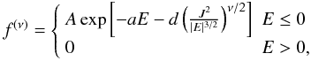 (A.4)
(A.4)
where A, a, d, and ν are positive constants, defining two scales and two dimensionless parameters. For applications, as described by Bertin & Trenti (2003), the dimensionless parameter ν can be fixed at ν = 1. Therefore, similarly to the King models, after integration of the relevant Poisson equation the f(ν) models are a one-parameter family of models, parametrized by their central concentration, which can be expressed by the central dimensionless potential Ψ = −aΦ(0).
The physical scales can be expressed as: 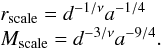 (A.5)By definition, these models are non-truncated and, because of this, are likely to be less suited to describe the outer parts of globular clusters. A study of globular clusters based on truncated f(ν) models is postponed to a separate investigation.
We recall that the surface brightness profiles for concentrated models (Ψ ≳ 7) are very close to de Vaucouleurs profile, while for low values of Ψ the models exhibit a sizeable core.
Appendix B: Fitting procedure
In the following we describe the procedure that we have adopted to perform the statistical analysis of the data. We basically follow Bertin et al. (1988).
B.1. Photometric fit
For each family of models considered in this paper, the photometric fit determines which equilibrium model has the projected mass distribution that best reproduces the surface brightness profile, under the assumption that:  (B.1)where Σ(R) is the model surface mass density, λ(R) the model surface luminosity density, and the mass-to-light ratio M/L is considered to be constant in the cluster. From the photometric data, we perform a fit that allows us to determine three parameters for each model:
-
Ψ, the concentration parameter, which determines the shape of the surface brightness and velocity dispersion profiles;
-
rs, the scale radius, that is r0 for the King models and rscale for the f(ν) models;
-
μ0, the central surface brightness.
We might determine the values of these parameters by minimizing the quantity:  (B.2)where S is the surface density expressed in magnitudes, but we found that it is more convenient to minimize:
  (B.3)because the chi-squared function turns out to be more stable, as pointed out by McLaughlin & van der Marel (2005). The connection between Eqs. (B.2) and (B.3) is easily made, by taking into account the following relations:
  (B.4)where the zero-point m0 = 26.422 allows us to express the observed surface brightness m(Ri) in solar units; the observed luminosities l(Ri) are expressed in solar units and δli are calculated from δmi and represent the errors on luminosities. The quantity
  is the surface density, normalized to its central value; from this point of view, the parameter k is related to the mass-to-light ratio.
Even if we calculated the parameters from the luminosities, we report the results in terms of magnitudes, because in this way a comparison with the data is more natural. To calculate the surface brightness profile μ(R) that best reproduces the data, we choose the model identified by Ψ, we calculate the normalized projected mass-density profile, and then we rescale it radially with rs and vertically with μ0.
Note that we have only two independent fit parameters, because k = k(Ψ,rs). Hence, the value of the reduced  is:
is:  (B.5)To have a quantitative estimate of the quality of the fit, it is convenient to calculate also the mean and maximum residuals:
  (B.6)
(B.6)
B.2. Kinematic fit
The parameters identified by the photometric fit determine a model, characterized by the parameter Ψ, the profiles of which are rescaled with rs. At this point, we perform a fit to the kinematic data to find the central line-of-sight velocity dispersion, that is the velocity scale needed to rescale vertically the normalized projected velocity dispersion profile calculated from the dynamical models. We calculate the value of this scale, V, as the one that minimizes:  (B.7)where σP(Ri) is the projected velocity dispersion calculated from the model, dependent on the rescaled radial coordinate. In this case, the values of the reduced χ2 and of the residuals can be found from the following expressions:
  (B.8)One might argue that a more sensible way to perform the fit would be by means of a single fit procedure, using the combined
  , defined as the sum of the photometric and of the kinematic contribution. We did perform tests of this different procedure and found that the results are equivalent to those obtained by performing the photometric fit first and then the kinematic fit at fixed Ψ and rs. This confirms the qualitative expectation that the kinematical data, being less numerous and less accurate with respect to the photometric ones, have little weight in determining Ψ and rs and are only needed to determine the scale V, that is, the relevant mass-to-light ratio.
Finally, we addressed the issue of whether a different representation of the results of the best-fit models would be more suitable than the one used in Figs. 1–3. Figure B.1 compares the appearance of a fit for a given object using a linear and a logarithmic representation of the radial scale. Based on this and other tests, we preferred to adopt a mixed representation, as used in the main text of the paper.
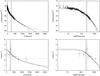 |
Fig. B.1
Linear vs. logarithmic representation for the photometric (upper panels) and kinematic (lower panels) profiles of NGC 6121. On the left, profiles are plotted with a linear radial scale, on the right with a logarithmic scale. |
| Open with DEXTER | |
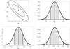 |
Fig. B.2
Confidence regions and confidence intervals on NGC 6121 King model parameters. The top left figure shows the overlap of the confidence regions, corresponding to confidence levels of 68.3% and 95.4% (solid lines), and the curves of constant χ2 (dashed lines); the black dot marks the position of the maximum of the likelihood (that is the minimum of χ2). The top right figure shows the confidence intervals for the likelihood depending on V; the bottom figures show the confidence intervals on the parameter Ψ and r0; the dark grey area corresponds to the confidence level of 68.3%, the light grey area to the confidence level of 95.4%; a solid vertical line marks the position of the maximum of the likelihood (that is the minimum of χ2). |
| Open with DEXTER | |
B.3. Goodness of the photometric and kinematic fits
To measure the goodness of the photometric and kinematic fits, we referred to the confidence intervals on the χ2-distribution. The probability density function of the χ2 distribution is defined as: 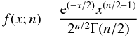 (B.9)when x ≥ 0, and zero otherwise. The parameter n corresponds to the number of degrees of freedom and Γ denotes the gamma function (e.g., see Abramowitz & Stegun 1972, Sect. 26.4).
The two-sided confidence interval relative to a confidence level α on the χ2 probability density function is defined as the interval  such that
 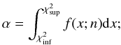 (B.10)and that:
  (B.11)
B.4. Errors on the best-fit parameters
For the methods described below, we refer mainly to Press et al. (2007). In the case of the photometric fit, we used the following procedure to calculate the formal errors on the parameters. First we calculated the Hessian matrix:  (B.12)where i = 1,2,3 and x1 = Ψ, x2 = rs and x3 = μ0; then we calculated the covariance matrix:
  (B.13)Finally, we obtained the errors: δxi = (Eii)1/2.
In the case of the kinematic fit, in which  depends analytically only on the parameter V, we can immediately calculate:
  (B.14)In addition to errors, we identified the relevant confidence regions and intervals for the various parameters, after defining a likelihood function Λ = e − χ2/2. First, we calculated confidence regions in the (Ψ,rs) plane, after marginalizing the likelihood function on k, in the following way:
  (B.15)We identified the regions corresponding to confidence levels of 68.3% and 95.4%. To check the results, we compared them with the regions defined by the curves of constant χ2 with the appropriate values (see Sect. 15.6 in Press et al. 2007). For each globular cluster and for the families of models, we notice that the regions identified with these two methods overlap in a consistent way.
We also calculated the confidence intervals on the parameters Ψ, rs and V (for the last parameter, the calculation can be done immediately, because the kinematic likelihood depends only on V; for the other parameters, we have to marginalize once more the likelihood function), corresponding to confidence levels of 68.3% and 95.4%. Comparing them with the errors calculated with the covariance matrix method, we found that the results are consistent.
In Fig. B.2 we show an example of the confidence regions and intervals calculated for the King best-fit model for the globular cluster NGC 6121. The top left panel shows the overlap of the confidence regions (solid lines) corresponding to confidence levels of 68.3% and 95.4%, and the curves of constant χ2 (dashed lines). It is clear that there is a good agreement between the two relevant pairs of curves. The bottom panels show the confidence intervals calculated on the marginalized likelihood for the parameters Ψ and r0, and the top right panel those for the parameter V; in these figures the confidence intervals are
shown as shaded areas. By comparing the extent of the dark grey area with the values of the uncertainties on the corresponding parameters (see Table 3), we see that the different methods lead to consistent results.
B.5. Derived parameters
Once the best-fit parameters have been secured, we may calculate other quantities, which represent some important characteristics of globular clusters.
In particular, for each family of models we calculated the core radius Rc, that is the radial position where the surface brightness equals half its central value, the half-mass radius rM, the total cluster mass M, the central mass density ρ0, the mass-to-light ratio M/L, the core relaxation time log Tc and the half-mass relaxation time, log TM. In addition, for King models we calculated the concentration parameter c and the truncation radius rtr. In turn, for the f(ν) models we calculated the anisotropy radius rα, defined as the radial position where α(rα) = 1, with  (B.16)The ratio of this radius to the half-mass radius measures how large is the radially-biased anisotropic part of the globular cluster: the smaller rα, the larger the anisotropic region of the cluster.
© ESO, 2012
Current usage metrics show cumulative count of Article Views (full-text article views including HTML views, PDF and ePub downloads, according to the available data) and Abstracts Views on Vision4Press platform.
Data correspond to usage on the plateform after 2015. The current usage metrics is available 48-96 hours after online publication and is updated daily on week days.
Initial download of the metrics may take a while.