| Issue |
A&A
Volume 526, February 2011
|
|
|---|---|---|
| Article Number | A105 | |
| Number of page(s) | 38 | |
| Section | Cosmology (including clusters of galaxies) | |
| DOI | https://doi.org/10.1051/0004-6361/201015830 | |
| Published online | 06 January 2011 | |
Online material
Appendix A: Luminosity cross-calibration
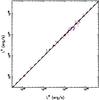 |
Fig. A.1
XMM-Newton-ROSAT vs. ROSAT-only measured luminosity in the 0.1–2.4 keV band within r500. The dashed line denotes 1:1. With a fixed slope to 1, the best-fit normalization of the XMM-Newton-ROSAT vs. ROSAT-only measured luminosity for the 62 clusters is 0.92 shown in solid line. The colors and symbols have the same meaning as those in Fig. 3. |
| Open with DEXTER | |
To cross-calibrate the XMM-Newton-ROSAT with the ROSAT-only measured X-ray luminosity, we re-derived the X-ray luminosity from ROSAT within r500 given in Sect. 2.2.1 by using the gas mass from the current work and the mass vs. gas mass relation in Pratt et al. (2009). The same spectral model was used to derive the X-ray luminosity using both ROSAT data alone and a combination of XMM-Newton and ROSAT data. The comparison between the XMM-Newton-ROSAT and ROSAT-only measured luminosity in the 0.1–2.4 keV band is shown in Fig. A.1.
The XMM-Newton-ROSAT to ROSAT-only measured luminosity ratio is (92 ± 2)%. The intrinsic scatter is (0.07 ± 0.01) dex. This was found for the REFLEX-DXL sample of 14 massive galaxy clusters at z ~ 0.3 in Zhang et al. (2006) and the REXCESS sample of 31 nearby galaxy clusters in Pratt et al. (2009,  ). The difference between the XMM-Newton-ROSAT and ROSAT-only measured luminosity is well within the intrinsic scatter.
Appendix B: Iron abundance vs. temperature
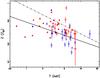 |
Fig. B.1
Iron abundance vs. temperature for the 62 clusters. The black line denotes our best power-law fit using the bisector method. The dot-dashed line is the best fit in Balestra et al. (2007) for clusters at higher redshifts (z ≥ 0.3) and in a higher temperature range (3–15 keV). The colors and symbols have the same meaning as those in Fig. 3. |
| Open with DEXTER | |
Appendix C: Scaling relations using Lin
In Table C.1, we present the X-ray bolometric luminosity within r500 ( ). We list the best fits to the corresponding scaling relations using the bolometric and 0.5–2 keV band luminosity in Table C.2, and show those plots using the bolometric luminosity in Figs. C.1–C.2, which helps us to understand the scatter driven by the presence of cool cores.
X-ray bolometric luminosity within r500, Lin, and in the [0.2 − 1] r500 annulus, Lex.
Power-law fit, log 10(Y) = A + Blog 10(X), to the scaling relations for the observational sample using Lin.
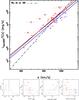 |
Fig. C.1
Upper panel: X-ray bolometric luminosity vs. velocity dispersion with luminosity derived from all emission interior to r500 ( |
| Open with DEXTER | |


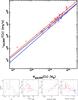 |
Fig. C.2
Upper panel: X-ray bolometric luminosity vs. gas mass with luminosity derived from all emission interior to r500 ( |
| Open with DEXTER | |

Appendix D: Scaling relations using Lex
Since the luminosity derived in the [0.2–1] r500 radial range is widely used to reduce the scatter caused by the presence of cool cores, we also present the X-ray bolometric luminosity in the [0.2–1] r500 radial range ( ) in Table C.1. We also list the best fits to the corresponding scaling relations using the bolometric and 0.5–2 keV band luminosity derived in the [0.2–1] r500 radial range in Table D.1, and show the plots using in Figs. D.1–D.2.
Power-law fit, log 10(Y) = A + Blog 10(X), to the scaling relations for the observational sample using Lex.
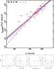 |
Fig. D.1
Upper panel: X-ray bolometric luminosity vs. velocity dispersion with luminosity derived from emission in the [0.2 − 1.0] r500 aperture ( |
| Open with DEXTER | |


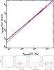 |
Fig. D.2
Upper panel: X-ray bolometric luminosity vs. gas mass with luminosity derived from emission in the [0.2 − 1.0] r500 aperture ( |
| Open with DEXTER | |

Appendix E: Scaling relations using 
We present the corresponding scaling relations using the 0.5–2 keV band luminosity corrected for the cluster central regions,  , in Figs. E.1–E.2. The best fits are listed in Table 3.
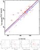 |
Fig. E.1
Upper panel: X-ray luminosity in the 0.5–2 keV band vs. velocity dispersion with luminosity corrected for the cluster core ( |
| Open with DEXTER | |


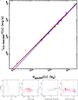 |
Fig. E.2
Upper panel: X-ray luminosity in the 0.5–2 keV band vs. gas mass with luminosity corrected for the cluster core ( |
| Open with DEXTER | |

Appendix F: XMM-Newton images of the sample
As the soft band is insensitive to the cluster temperature and has data of high signal-to-noise ratio, we use the MOS and pn combined image in the 0.7–2 keV band to illustrate the X-ray morphological substructure of each cluster (Figs. F.1–F.5). X-ray point-like sources are identified and subtracted. The holes, where the point-like sources were, are re-filled with the Chandra CIAO routine “dmfilth” using randomization based on the surface brightness distribution around the holes. We only use this image to demonstrate the existence of morphological substructure in the cluster. Significant substructure features shown in the image are excised before we perform the spectral and surface brightness analysis.
As addressed in Sect. 2.3, 13 of the 16 clusters with large offsets between the X-ray flux-weighted centers (see Table 1) and BCG positions are disturbed clusters (see Table 2). We now comment on these 13 clusters. The BCGs in A0399 and A1736 are slightly offset from the main X-ray emission. The ICM in A3376, A0754, A2256, and A3667 exhibits a comet-like tail, and their BCGs are at the opposite end from the X-ray centers probably because of their on-going dynamical activity. A3395s is the south component of a bi-cluster, and its BCG is at an X-ray weak bright peak. The ICM in A1367 has multi-peaks, and the BCG is at the northwest X-ray peak, which is not the brightest one. The BCG in A2163 (A2255) is not a dominant BCG, which sits slightly east (west) of the X-ray center. This also applies but less significantly to some more clusters in the sample. The ICM in Coma, A3558, and A2065 shows some weakly disturbed features, and their BCGs are only 40–60 kpc away from the X-ray centers. A3158, A3391, and A0576 are relaxed clusters, and their BCGs are ≳40 kpc away from the X-ray centers.
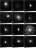 |
Fig. F.1
Combined MOS and pn images of the clusters in the 0.7–2 keV band, where point sources have been excised and refilled with values from neighboring pixels. |
| Open with DEXTER | |
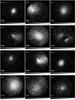 |
Fig. F.2
Combined MOS and pn images of the clusters in the 0.7–2 keV band, where point sources have been excised and refilled with values from neighboring pixels. |
| Open with DEXTER | |
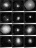 |
Fig. F.3
Combined MOS and pn images of the clusters in the 0.7–2 keV band, where point sources have been excised and refilled with values from neighboring pixels. |
| Open with DEXTER | |
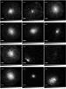 |
Fig. F.4
Combined MOS and pn images of the clusters in the 0.7–2 keV band, where point sources have been excised and refilled with values from neighboring pixels. |
| Open with DEXTER | |
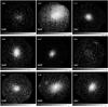 |
Fig. F.5
Combined MOS and pn images of the clusters in the 0.7–2 keV band, where point sources have been excised and refilled with values from neighboring pixels. |
| Open with DEXTER | |
Appendix G: Systematic errors in estimates of σ
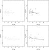 |
Fig. G.1
Velocity dispersion measured by the 45 most massive galaxies normalized by the velocity dispersion within 1.2 Abell radii as a function of the fraction of galaxies for the simulated sample. The results are only based on the simulated sample of the 21 clusters. The colors and symbols have the same meaning as those in Fig. 10. The curves are the local regression non-parametric fits. |
| Open with DEXTER | |
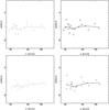 |
Fig. G.2
Velocity dispersion measured by the 45 most massive galaxies normalized by the velocity dispersion within 1.2 Abell radii as a function of velocity dispersion for the simulated sample. The results are only based on the simulated sample of the 21 clusters. The colors and symbols have the same meaning as those in Fig. 10. The curves are the local regression non-parametric fits. |
| Open with DEXTER | |
© ESO, 2011
Current usage metrics show cumulative count of Article Views (full-text article views including HTML views, PDF and ePub downloads, according to the available data) and Abstracts Views on Vision4Press platform.
Data correspond to usage on the plateform after 2015. The current usage metrics is available 48-96 hours after online publication and is updated daily on week days.
Initial download of the metrics may take a while.