| Issue |
A&A
Volume 503, Number 3, September I 2009
|
|
|---|---|---|
| Page(s) | 691 - 706 | |
| Section | Cosmology (including clusters of galaxies) | |
| DOI | https://doi.org/10.1051/0004-6361/200911624 | |
| Published online | 27 May 2009 | |
Online Material
Appendix A: Parameterisation the foreground component and choice of a mask
In this appendix, we discuss in more detail the dimension D of matrix used to represent the covariance of the total galactic emission, and the choice of a mask to hide regions of strong galactic emission for the estimation of r with SMICA.
A.1 Dimension D of the foreground component
First, we explain on a few examples the mechanisms which set the rank
of the foreground covariance matrix, to give an intuitive
understanding of how the dimension D of the foregrounds component
used in SMICA to obtain a good model of the data. Let us consider
the case of a ``perfectly coherent'' physical process, for which the
total emission, as a function of sky direction ![]() and frequency
and frequency ![]() ,
is well described by a spatial template multiplied by a
pixel-independent power law frequency scaling:
,
is well described by a spatial template multiplied by a
pixel-independent power law frequency scaling:
The covariance matrix of this foreground will be of rank one and
This is not necessarily the best linear approximation of the emission, but supposing it holds, the covariance matrix of the foreground will be of rank two (as the sum of two correlated rank 1 processes). If the noise level is sufficiently low, the variation introduced by the first order term of Eq. (A.2) becomes truly significant, we can't model the emission by a mono-dimensional component as in Eq. (A.1).
In this work, we consider two processes, synchrotron and dust, which are expected to be correlated (at least by the galactic magnetic field and the general shape of the galaxy). Moreover, significant spatial variation of their emission law arises (due to cosmic aging, dust temperature variation ...), which makes their emission only partially coherent from one channel to another. Consequently, we expect that the required dimension D of the galactic foreground component will be at least 4 as soon as the noise level of the instrument is low enough.
The selection of the model can also be made on the basis of a statistical criterion. For example, Table A.1 shows the Bayesian information criterion (BIC) in the case of the EPIC-2m experiment (r = 0.01) for 3 consecutive values of D. The BIC is a decreasing function of the likelihood and of the number of parameter. Hence, lower BIC implies either fewer explanatory variables, better fit, or both. In our case the criterion reads:
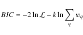
where k is the number of estimated parameters and wq the effective number of modes in bin q. Taking into account the redundancy in the parameterisation, the actual number of free parameters in the model is
Table A.1: Bayesian information criterion of 3 models with increasing dimension of the galactic component for the EPIC-2m mission.
A.2 Masking influence
The noise level and the scanning strategy remaining fixed in the full-sky experiments, a larger coverage gives more information and should result in tighter constraints on both foreground and CMB. In practice, it is only the case up to a certain point, due to the non stationarity of the foreground emission. In the galactic plane, the emission is too strong and too complex to fit in the proposed model, and this region must be discarded to avoid contamination of the results. The main points governing the choice of an appropriate mask are the following:
- the covariance of the total galactic emission (synchrotron and dust polarised emissions), because of the variation of emission laws as a function of the direction on the sky, is never exactly modelled by a rank D matrix. However it is satisfactorily modelled in this way if the difference between the actual second order statistics of the foregrounds, and those of the rank D matrix model, are indistinguishable because of the noise level (or because of cosmic variance in the empirical statistics). The deviation from the model is more obvious in regions of strong galactic emission, hence the need for a galactic mask. The higher the noise, the smaller the required mask;
- SMICA provides a built-in measure of the adequacy of the model, which is the value of the spectral mismatch. If too high, the model under-fits the data, and the dimension of the foreground model (or the size of the mask) should be increased. If too low, the model over-fits the data, and D should be decreased;
- near full sky coverage is better for measuring adequately the reionisation bump;
- the dimension of the foreground component must be smaller than the number of channels.
If, on the other hand, the error seems dominated by the contribution of foregrounds, which is, for example, the case of the EPIC-2m experiment for r = 0.001, the tradeoff is unclear and it may happen that a better estimator is obtained with a stronger masking of the foreground contamination. We found that it is not the case. Table A.2 illustrates the case of the EPIC-2m experiment with the galactic cut used in Sect. 4 and a bigger cut. Although the reduction of sensitivity is slower in the presence of foreground than for the noise dominated case, the smaller mask still give the better results.
Table A.2: Estimation of the tensor to scalar ratio with two different galactic cuts in the EPIC-2m experiment.
We may also recall that the expression (7) of the likelihood is an approximation for partial sky coverage. The scheme presented here thus may not give fully reliable results when masking effects become important.
Appendix B: Spectral mismatch
Computed for each bin q of ![]() ,
the mismatch criterion,
,
the mismatch criterion,
![]() ,
between the best-fit model
,
between the best-fit model
![]() at the point of convergence
at the point of convergence ![]() ,
and the data
,
and the data
![]() ,
gives a picture of the goodness of fit as a function of the
scale. Black curves in Figs. B.1 and B.2 show the mismatch criterion of the best fits for
Planck and EPIC designs respectively. When the model holds, the value
of the mismatch is expected to be around the number of degrees of
freedom (horizontal black lines in the figures). We can also compute
the mismatch for a model in which we discard the CMB contribution
,
gives a picture of the goodness of fit as a function of the
scale. Black curves in Figs. B.1 and B.2 show the mismatch criterion of the best fits for
Planck and EPIC designs respectively. When the model holds, the value
of the mismatch is expected to be around the number of degrees of
freedom (horizontal black lines in the figures). We can also compute
the mismatch for a model in which we discard the CMB contribution
![]() .
Gray curves in
Figs. B.1 and B.2 show the mismatch
for this modified model. The difference between the two curves
illustrates the ``weight'' of the CMB component in the fit, as a
function of the scale.
.
Gray curves in
Figs. B.1 and B.2 show the mismatch
for this modified model. The difference between the two curves
illustrates the ``weight'' of the CMB component in the fit, as a
function of the scale.
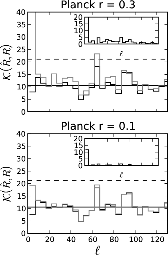 |
Figure B.1:
Those plots present the distribution in |
| Open with DEXTER | |
Figure B.1 shows the results for Planck for
r=0.3 and 0.1. The curves of the difference plotted in inclusion
illustrate the predominance of the reionisation bump. In
Fig. B.2, we plot the difference curve on the bottom
panels for the three experiments for r=0.01 and r=0.001. They
illustrate clearly the difference of sensitivity to the peak between
the EPIC-LC design and the higher resolution experiments. In general
it can be seen that no significant contribution to the CMB is coming
from scales smaller than
![]() .
.
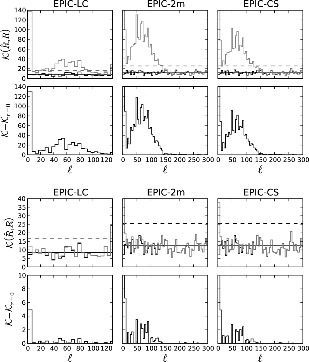 |
Figure B.2:
Mismatch criterion for r = 0.01 ( top) and r = 0.001
( bottom). In each plot, the top panel shows the mismatch criterion between the best fit model and the data (black curve) and the best fit model deprived from the CMB contribution and the data (gray curve). Solid and dashed horizontal lines show respectively the mismatch expectation and 2 times the mismatch expectation. The difference between the gray and the black curve is plotted in the bottom panel and gives an idea of the significance of the CMB signal in each bin of |
| Open with DEXTER | |
Current usage metrics show cumulative count of Article Views (full-text article views including HTML views, PDF and ePub downloads, according to the available data) and Abstracts Views on Vision4Press platform.
Data correspond to usage on the plateform after 2015. The current usage metrics is available 48-96 hours after online publication and is updated daily on week days.
Initial download of the metrics may take a while.