© The Authors 2026

1. Introduction

The magnetic field is the main driver of activity in the upper solar atmosphere, but its quantitative determination above the photosphere remains a major challenge in solar physics (see, e.g., Wiegelmann et al. 2014; de la Cruz Rodríguez & Leenaarts 2024). With respect to the chromosphere, prominences, spicules, filaments, and coronal structures, the interpretation of polarized spectral lines generally requires a quantitative description of several atomic processes, including anisotropic radiation pumping, atomic polarization, the Hanle effect, and collisional effects (e.g., Hanle 1924; Sahal-Bréchot 1977; Stenflo 1994; Landi Degl’Innocenti & Landolfi 2004; Derouich 2020).

Among the most important diagnostics of the outer solar atmosphere, there are the neutral helium multiplets at 10830 Å (2s ³S → 2p ³P°) and at 5876 Å, the D₃ line (2p ³P° →3d ³D). These lines are observed both on the disk and off the limb, and their polarization is sensitive to magnetic fields from fractions of a gauss to several hundred gauss, a range highly relevant for prominences, filaments, spicules, active-region chromospheres, and eruptive structures (e.g., Trujillo Bueno et al. 2002; Casini et al. 2003; Asensio Ramos et al. 2008; Trujillo Bueno & del Pino Alemán 2022). The metastable lower term of the He I10830 Å multiplet makes this line especially useful for probing the upper chromosphere, while the D₃ line provides a complementary diagnostic in off-limb plasma.

Recent observations further illustrate the diagnostic relevance of these helium lines. High-sensitivity He I D₃ spectropolarimetry with ZIMPOL-3 at IRSOL has been used to infer the magnetic and thermodynamic structure of an active-region prominence (e.g., Esteban Pozuelo et al. 2025), while imaging spectropolarimetry in the He I10830 Å triplet has revealed high-speed flows and transition-region-like temperatures during flux emergence (e.g., Leenaarts et al. 2025). Current facilities, such as DKIST, together with planned next-generation facilities such as EST, will provide increasingly sensitive visible and near-infrared spectropolarimetry of the chromosphere and low corona (e.g., Rimmele et al. 2020; Quintero Noda et al. 2022), making reliable collisional rates for He I polarization modeling increasingly important.

The development of quantum-mechanical modeling, polarized radiative-transfer calculations, and inversion techniques has progressively established the He I D₃ and 10830 Å multiplets as standard tools for diagnosing magnetic fields in the solar atmosphere. Early theoretical studies of scattering polarization and the Hanle effect in the He I D₃ line demonstrated its diagnostic potential for prominence magnetic fields (e.g., Bommier & Sahal-Bréchot 1978; Landi Degl’Innocenti 1982). This diagnostic framework was subsequently extended and applied to a wide variety of solar structures, including prominences and filaments, spicules, and active-region chromospheres (e.g., López Ariste & Casini 2002; Trujillo Bueno et al. 2002, 2005; Casini et al. 2003; Merenda et al. 2006; Kuckein et al. 2009, 2020; Centeno et al. 2010; Sasso et al. 2011; Orozco Suárez et al. 2014; Schad et al. 2016; Díaz Baso et al. 2019; Anan et al. 2021). However, one physical ingredient remains insufficiently constrained: the role of elastic collisions with neutral hydrogen. Vicente Arévalo et al. (2023) pointed out that such collisions are usually assumed to produce only weak depolarization of He I under typical chromospheric and prominence conditions, but also emphasized that this assumption has not been investigated in detail and might need to be tested in sufficiently dense active-region filaments.

In polarized non-LTE (NLTE) modeling, isotropic collisions with neutral hydrogen enter the statistical equilibrium equations (SEE) together with radiative and magnetic terms. They can relax the multipole moments of the atomic density matrix, including the alignment responsible for linear polarization, and can transfer population and polarization between fine-structure levels or between coherences. Their importance depends on the local plasma conditions and on their competition with radiative and magnetic processes. Therefore, even when collisions are expected to be weak in many prominence or chromospheric conditions, quantitative rates are required to assess this assumption, rather than impose it a priori.

A general theoretical framework for collisions with neutral hydrogen has been developed over several decades. The Anstee-Barklem-O’Mara (ABO) theory of collisional line broadening (e.g., Anstee & O’Mara 1991; Anstee & O’Mara 1995; Barklem & O’Mara 1997; Barklem et al. 1998) was extended to the depolarization and polarization-transfer problem by Derouich, Sahal-Bréchot, Barklem (DSB), and collaborators (e.g., Derouich et al. 2003a,b, 2004a,b, 2005b, 2006; Sahal-Bréchot et al. 2007; Derouich 2020). Derouich (2020) summarized extensive calculations for simple atoms in p-, d-, and f-states into analytical variation laws as functions of the effective principal quantum number n^*, while Derouich et al. (2005b) treated s states.

In the present work, we adopted a frozen-core approximation in which the inner 1s electron is treated as a core with total angular momentum, J_c = 1/2, while the outer electron is treated as the active valence electron. The collision with neutral hydrogen is assumed to act mainly on this valence electron, with the core angular momentum conserved during the collision. This makes it possible to construct He I collisional rates from simple-atom rates by means of angular-momentum recoupling relations involving Wigner 9j symbols. A similar approach was also applied when calculating hyperfine structure rates via calculation of fine-structure rates (see, e.g., Nienhuis 1976; Omont 1977; Derouich 2020), where a frozen-nuclear-spin approximation was adopted.

The adopted helium atomic model includes the low-lying singlet and triplet terms relevant for the main solar He I diagnostics: 1s2s ³S, 1s2p ³P, 1s2p ¹P, 1s3s ³S, 1s3p ³P, 1s3p ¹P, 1s3d ³D, and 1s3d ¹D, with the corresponding fine-structure levels resolved where applicable. The singlet and triplet systems are treated within the same model to provide a more complete atomic description and to facilitate future extensions that include inelastic processes, such as electron-impact excitation, capable of coupling the two systems.

The aim of this paper is to provide collisional depolarization, polarization-transfer, and population-transfer rates for He I levels due to isotropic collisions with neutral hydrogen. The paper is organized as follows. Section 2 describes the effect of isotropic collisions on the atomic density matrix and introduces the coupling scheme used to construct the He I rates. Section 3 presents the extension from the multilevel to the multiterm formulation. Section 4 explains how the rates are inferred from simple-atom variation laws and gives the resulting tables. Section 5 summarizes the main conclusions.

2. Effect of isotropic collisions on the atomic polarization

2.1. Density-matrix elements and collisional contribution

In the density-matrix formalism (e.g., Blum 1981; Landi Degl’Innocenti & Landolfi 2004), the excitation state of an atomic level (α 𝒥) is described by the statistical tensors, ${\rho }_q^{k_{\mathcal{J}}}(\alpha \mathcal{J})$. The multipole of rank k_𝒥 = 0 represents the population of the level, odd ranks, in particular k_𝒥 = 1, describe orientation, and even ranks with k_𝒥 > 0, in particular k_𝒥 = 2, describe alignment-type atomic polarization. The linear polarization is directly related to the alignment components, while the circular polarization is related to the orientation components (e.g., Landi Degl’Innocenti & Landolfi 2004). In the case where the emitting atom is excited by anisotropic but unpolarized radiation, only even values of k_𝒥 are directly created, following the usual optical-pumping selection rules, implying that only linear polarization is observed.

Isotropic collisions with neutral hydrogen modify the atomic polarization because they tend to equalize the populations of the Zeeman sublevels and to destroy the coherences between them (e.g., Derouich et al. 2003a,b). In other words, collisions act directly on the density-matrix elements and, as a consequence, on the polarization of the emergent radiation. Under the impact approximation, collisions are assumed to be binary, complete, and well separated in time, so that the collisional rates are proportional to the hydrogen density, n_H.

In a multilevel atom, the SEE are obtained by including all the relevant processes that intervene during line formation. The relative importance of these processes depends on the physical conditions of the medium where the line is formed. In solar applications, it is generally necessary to take into account radiative, magnetic, and collisional contributions. In the stationary regime, we have

$$\begin{array}{c}\hfill {\left(\frac{d}{\mathit{dt}}{\rho }_q^{k_{\mathcal{J}}}(\alpha \mathcal{J})\right)}_{\mathrm{rad}}+{\left(\frac{d}{\mathit{dt}}{\rho }_q^{k_{\mathcal{J}}}(\alpha \mathcal{J})\right)}_{\mathrm{mag}}+{\left(\frac{d}{\mathit{dt}}{\rho }_q^{k_{\mathcal{J}}}(\alpha \mathcal{J})\right)}_{\mathrm{coll}}=0.\end{array}$$(1)

If collisions are neglected or if the corresponding collisional rates are poorly known, part of the information encoded in the spectropolarimetric observations may be lost or misinterpreted. In particular, since the magnetic field is often one of the main unknowns of the SEE, uncertainties in the collisional terms can propagate directly into the inferred magnetic field and lead to an inaccurate determination of its strength and orientation.

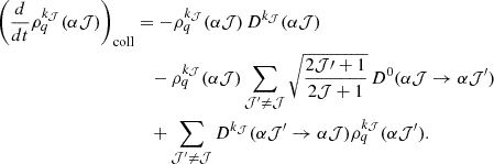
For a level (α 𝒥), the collisional contribution to the SEE (see, e.g., Sahal-Bréchot et al. 2007; Derouich 2020) can be written as

$$\begin{array}{cc}\hfill {\left(\frac{d}{\mathit{dt}}{\rho }_q^{k_{\mathcal{J}}}(\alpha \mathcal{J})\right)}_{\mathrm{coll}}& =-{\rho }_q^{k_{\mathcal{J}}}(\alpha \mathcal{J})D^{k_{\mathcal{J}}}(\alpha \mathcal{J})\hfill \\ \hfill & -{\rho }_q^{k_{\mathcal{J}}}(\alpha \mathcal{J}){\displaystyle \sum _{{\mathcal{J}}^{\prime }\ne \mathcal{J}}}\sqrt{\frac{2\mathcal{J}\prime +1}{2\mathcal{J}+1}}{D}^0(\alpha \mathcal{J}\to \alpha {\mathcal{J}}^{\prime })\hfill \\ \hfill & +{\displaystyle \sum _{{\mathcal{J}}^{\prime }\ne \mathcal{J}}}{D}^{k_{\mathcal{J}}}(\alpha {\mathcal{J}}^{\prime }\to \alpha \mathcal{J}){\rho }_q^{k_{\mathcal{J}}}(\alpha {\mathcal{J}}^{\prime }).\hfill \end{array}$$(2)

The first term on the right-hand side represents the relaxation of the multipole, ${\rho }_q^{k_{\mathcal{J}}}(\alpha \mathcal{J})$. via collisions, whereas the second one describes the transfer of polarization from (α𝒥′) toward the level (α𝒥). Since the collisions are isotropic, all the components q of a given tensorial rank, k_𝒥, are affected in the same way.

The quantity $D^{k_{\mathcal{J}}}(\alpha \mathcal{J})$ is the collisional depolarization rate of rank, k_𝒥, for the level (α𝒥). For purely elastic collisions, the population of the level is conserved, so that D⁰(α𝒥) = 0. We note that for k_𝒥 = 0, we have the population-transfer rate, D⁰(α𝒥 → α𝒥′). The polarization-transfer rate of rank k_𝒥 from (α𝒥) to (α𝒥′) is denoted as $D^{k_{\mathcal{J}}}(\alpha \mathcal{J}\to \alpha \mathcal{J}\prime )$. The total rank-k_𝒥 relaxation rate of the level (α𝒥) is the sum of $D^{k_{\mathcal{J}}}(\alpha \mathcal{J})$ and the transfer rate contribution, ${\displaystyle \sum _{\mathcal{J}\prime \ne \mathcal{J}}}\sqrt{(2\mathcal{J}\prime +1)/(2\mathcal{J}+1)}{D}^0(\alpha \mathcal{J}\to \alpha \mathcal{J}\prime )$.

2.2. Coupling scheme

The He I atom has two electrons. For the singly excited states considered in this work, one electron remains in the 1s shell, while the second electron occupies an nl orbital. We used the frozen-core approximation, in which the inner 1s electron is treated as a core and the outer electron is treated as the active valence electron. Within the frozen-core approximation (see, e.g., Derouich et al. 2005a; Derouich 2020), the singly excited He I is described by assuming that one electron remains in the 1s shell and forms the frozen core, while the second electron in the nl orbital is treated as the active valence electron. The collision with neutral hydrogen is assumed to affect only this outer electron, whose orbital and spin angular momenta are l and s = 1/2, respectively. As a consequence, the core angular momentum is conserved during the collision, while the depolarization and polarization-transfer rates for He I can be expressed as linear combinations of the corresponding rates for a simple atom associated with the external nl electron. The relevant coupling scheme is defined by the valence-electron angular momenta, l and s, its total angular momentum, j = l + s, the core angular momenta, L_c and S_c, the core total angular momentum, J_c = L_c + S_c, and the total atomic angular momentum, 𝒥 = J_c+j. For all He I levels considered here, the core corresponds to the 1s²S_1/2 electron, so that L_c = 0, S_c = 1/2, and J_c = 1/2.

These levels can be treated with Eqs. (3) and (5), where (α𝒥) denotes the He I level under consideration. In this picture, the inner 1s electron defines the core, whereas the outer electron is treated as the valence (or optical) electron. We adopted a He I model atom including the lowest singlet and triplet terms arising from the configurations 1s², 1s 2s, 1s 2^p, 1s 3^s, 1s 3^p, and 1s 3^d, with the relevant fine-structure 𝒥-levels resolved for polarization and magnetic diagnostics. The model comprises the ground state 1s^{2 1}S₀; the n = 2 terms 1s 2s ³S₁, 1s 2s ¹S₀, 1s 2p ³P_𝒥 (𝒥 = 0,1,2), and 1s 2p ¹P₁; and the n = 3 terms 1s 3s ³S₁, 1s 3s ¹S₀, 1s 3p ³P_𝒥 (𝒥 = 0,1,2), 1s 3p ¹P₁, 1s 3d ³D_𝒥 (𝒥 = 1,2,3), and 1s 3d ¹D₂. This term structure contains the triplet manifold responsible for the principal He I diagnostic lines; in particular, the 10 830 Å transition (2s ³S₁ → 2p ³P_𝒥), the D₃ 5876 Å transition (2p ³P_𝒥 → 3d ³D_𝒥), as well as the 7065 Å and 3889 Å lines. Under chromospheric and prominence conditions, the long-lived metastable 2s ³S₁ level efficiently populates the triplet ladder. Thus, this model atom offers a standard framework for describing the polarization of the strongest He I triplet lines in solar applications.

The complete set of quantum numbers used in the multilevel formulation is summarized in Table 1. This table specifies, for each configuration and term included in the adopted He I atomic model: the values of L, S, the fine-structure levels, 𝒥′ and 𝒥, the valence-electron orbital angular momentum l, the contributing valence-electron channels, j′ (final level) and j (initial level), and the allowed even tensorial ranks, k_𝒥. It therefore provides the angular-momentum basis required for applying the frozen-core recoupling relations in Eqs. (3) and (5) and for constructing the collisional depolarization and polarization-transfer rates used throughout this work. For the depolarization rates, the two levels coincide (𝒥 = 𝒥′, j′=j). For the transfer rates (𝒥 ≠ 𝒥′), the table lists only the off-diagonal channels with j ≠ j′ and a diagonal channel, j = j′, does not contribute to a complex-atom transfer rate.

The singlet terms included in this work, together with their depolarization and polarization-transfer rates, were also calculated. Indeed, when inelastic collisions are included (especially electron-impact excitation), the assumption of a purely triplet model might become overly restrictive. Although singlet-triplet radiative transitions are forbidden, singlet terms can still influence the triplet terms populations and polarizations through collisional coupling (population transfer and polarization transfer) between the two spin systems. For this reason, we extended the commonly adopted triplet scheme by explicitly including additional low-lying singlet terms alongside the corresponding triplet terms. This yields a more flexible and physically complete multiterm atomic model whenever inelastic electron collisions are accounted for and it reduces the risk of bias in the inferred polarization signals when singlet-triplet collisional channels are non-negligible under chromospheric conditions.

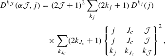
By assuming that the core of the He I atom is frozen, the collisional depolarization rate of a level (α𝒥) of a complex atom can be written following Derouich (2020), as

$$\begin{array}{cc}\hfill D^{k_{\mathcal{J}}}(\alpha \mathcal{J},j)& ={(2\mathcal{J}+1)}^2{\displaystyle \sum _{k_j}}(2k_j+1)D^{k_j}(j)\hfill \\ \hfill & \times {\displaystyle \sum _{k_{J_c}}}(2k_{J_c}+1){\left\{\begin{array}{ccc}j& J_c& \mathcal{J}\\ j& J_c& \mathcal{J}\\ k_j& k_{J_c}& k_{\mathcal{J}}\end{array}\right\}}^2,\hfill \end{array}$$(3)

where J_c is the total angular momentum of the core, j is the total angular momentum of the external valence electron, and D^k_j(j) is the depolarization rate of the external shell treated as that of a simple atom. The quantities k_j, k_Jc, and k_𝒥 are the tensorial ranks. When two j-channels contribute additively to the same level (α𝒥) (as can be seen in Table 1), the depolarization rate is obtained by summing the corresponding contributions,

$$\begin{array}{c}\hfill D^{k_{\mathcal{J}}}(\alpha \mathcal{J})={\displaystyle \sum _j}{D}^{k_{\mathcal{J}}}(\alpha \mathcal{J},j).\end{array}$$(4)

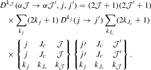
Similarly, the polarization-transfer rates between fine-structure levels (α𝒥) and (α𝒥′) are given by (see, e.g., Derouich 2020)

$$\begin{array}{cc}& D^{k_{\mathcal{J}}}(\alpha \mathcal{J}\to \alpha {\mathcal{J}}^{\prime },j,j^{\prime })=(2\mathcal{J}+1)(2{\mathcal{J}}^{\prime }+1)\hfill \\ & \times {\displaystyle \sum _{k_j}}(2k_j+1)D^{k_j}(j\to j^{\prime }){\displaystyle \sum _{k_{J_c}}}(2k_{J_c}+1)\hfill \\ & \times \left\{\begin{array}{ccc}j& J_c& \mathcal{J}\\ j& J_c& \mathcal{J}\\ k_j& k_{J_c}& k_{\mathcal{J}}\end{array}\right\}\left\{\begin{array}{ccc}j\prime & J_c& {\mathcal{J}}^{\prime }\\ j\prime & J_c& {\mathcal{J}}^{\prime }\\ k_j& k_{J_c}& k_{\mathcal{J}}\end{array}\right\}.\hfill \end{array}$$(5)

Summing over all valence-electron channels compatible with the initial and final He I fine-structure levels, with j ≠ j′ (diagonal channels do not contribute to a transfer), yields the total multilevel transfer rate of

$$\begin{array}{c}\hfill D^{k_{\mathcal{J}}}(\alpha \mathcal{J}\to \alpha {\mathcal{J}}^{\prime })={\displaystyle \sum _{\begin{array}{c}(j,j\prime )\\ j\ne j^{\prime }\end{array}}}{D}^{k_{\mathcal{J}}}(\alpha \mathcal{J}\to \alpha {\mathcal{J}}^{\prime },j,j^{\prime }).\end{array}$$(6)

For s-states, l = 0, and only $j=\frac{1}{2}$ is possible. For p-states, l = 1, and the possible channels are $j=\frac{1}{2},\frac{3}{2}$.

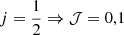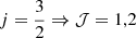Since $J_c=\frac{1}{2}$, these channels give $j=\frac{1}{2}\Rightarrow \mathcal{J}=0,1$ and $j=\frac{3}{2}\Rightarrow \mathcal{J}=1,2$. Thus, the level 𝒥 = 1 can receive contributions from both $j=\frac{1}{2}$ and $j=\frac{3}{2}$. For d-states, l = 2, and the possible channels are $j=\frac{3}{2},\frac{5}{2}$.

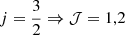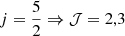These expressions give $j=\frac{3}{2}\Rightarrow \mathcal{J}=1,2$; and $j=\frac{5}{2}\Rightarrow \mathcal{J}=2,3$. Thus, the level 𝒥 = 2 can receive contributions from both $j=\frac{3}{2}$ and $j=\frac{5}{2}$.

For a given He I level, the collision rate is first evaluated for each allowed valence-electron channel, j, and the partial contributions are then added. Thus, levels admitting a single j channel, such as s-states, have a single contribution, whereas the levels 𝒥 = 1 in p-states and 𝒥 = 2 in d-states require a sum over the two allowed channels. The same rule is used for transfer rates.

The complex-atom polarization- and population-transfer rate $D^{k_{\mathcal{J}}}(\alpha \mathcal{J}\to \alpha \mathcal{J}\prime )$ is, by construction, a recoupling of the simple-atom transfer rate D^k_j(j → j′) with j ≠ j′. Therefore, a valence-electron channel contributes to the complex-atom transfer rate only if the corresponding simple-atom transfer rate D^k_j(j → j′) actually exists. This same constraint applies to the multiterm transfer rates introduced below. By contrast, the multilevel depolarization rates D^k_𝒥(α𝒥) and the multiterm depolarization rates discussed in the next section involve the simple-atom depolarization rate D^k_j(j), corresponding to the diagonal case, j = j′.

General laws were obtained in Derouich et al. (2005b) for a valence electron in s-states and in Derouich (2020) for a valence electron in p- and d-states; these laws allow us to calculate D^k_j(j) and D^k_j(j → j′), which can then be used to infer the collisional rates needed for modeling the polarization of He I lines. For each fine-structure level involved in the He I atomic model, the effective principal quantum number, n^*, is first determined from the known atomic energy levels.

3. Multiterm formulation and statistical equilibrium equations

In the multilevel formulation, the atomic polarization is described by the statistical tensors ${\rho }_q^k(\alpha \mathcal{J})$, where each fine-structure level (α𝒥) is treated separately. A more general treatment of scattering polarization can be obtained via the multiterm framework (e.g., Landi Degl’Innocenti & Landolfi 2004), which allows for coherences not only between Zeeman sublevels of a given 𝒥-level, but also between different 𝒥-levels belonging to the same LS term, α ≡ (n l L S). In this case the atomic polarization is described by spherical statistical tensors, ${\rho }_q^{k_{\mathcal{J}}}(\alpha \mathcal{J}\mathcal{J}\prime )$, which include both diagonal (𝒥 = 𝒥′) and off-diagonal (𝒥 ≠ 𝒥′) elements.

The diagonal elements with 𝒥 = 𝒥 ′ describe the population and polarization of a given fine-structure level, while the off-diagonal elements with 𝒥 ≠ 𝒥 ′ describe coherences between different fine-structure levels of the same term. The allowed tensorial ranks satisfy

$$|\mathcal{J}-\mathcal{J}\prime |\le k_{\mathcal{J}}\le \mathcal{J}+\mathcal{J}\prime .$$

In the present work, only even values of k were retained, since they serve as the relevant ranks for population and linear-polarization studies. The rank k_𝒥 = 0 corresponds to population, while k_𝒥 = 2 corresponds to alignment. Higher even ranks, such as k_𝒥 = 4 and k_𝒥 = 6, are also retained when possible because they could be coupled to the lower ranks through the SEE.

In the multiterm case, isotropic collisions contribute to the SEE through a relaxation of ${\rho }_q^{k_{\mathcal{J}}}(\alpha \mathcal{J}\mathcal{J}\prime )$ and through a transfer-term coupling of different pairs (𝒥, 𝒥′) and (𝒥″, 𝒥″′) within the same term. The collisional contribution (e.g., Derouich & Qutub 2024) can be expressed as

$$\begin{array}{cc}\hfill {\left(\frac{d}{\mathit{dt}}{\rho }_q^{k_{\mathcal{J}}}(\alpha JJ\prime )\right)}_{\mathrm{coll}}& =-[D^{k_{\mathcal{J}}}(\alpha JJ\prime )+{\displaystyle \sum _{(J″J\prime ″)\ne (JJ\prime )}}\sqrt{\frac{J″+J\prime ″+1}{J+J\prime +1}}\hfill \\ \hfill & \times D^0(\alpha JJ\prime \to \alpha J″J\prime ″)]{\rho }_q^{k_{\mathcal{J}}}(\alpha JJ\prime )\hfill \\ \hfill & +{\displaystyle \sum _{(J″J\prime ″)\ne (JJ\prime )}}{D}^{k_{\mathcal{J}}}(\alpha J″J\prime ″\to \alpha JJ\prime ){\rho }_q^{k_{\mathcal{J}}}(\alpha J″J\prime ″),\hfill \end{array}$$(7)

where $D^{k_{\mathcal{J}}}(\alpha \mathcal{J}\mathcal{J}\prime )$ represents the rank-k_𝒥 collisional relaxation of the coherence (𝒥, 𝒥′) and $D^{k_{\mathcal{J}}}(\alpha \mathcal{J}\mathcal{J}\prime \to \alpha \mathcal{J}″\mathcal{J}″)$ are the polarization- and/or population-transfer rates between pairs of fine-structure levels within the term.

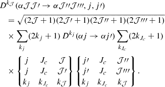
Direct computations of the full set of multiterm rates, $D^{k_{\mathcal{J}}}(\alpha \mathcal{J}\mathcal{J}\prime )$ and D^k_𝒥(α𝒥𝒥′→α𝒥″𝒥^″′), are generally difficult because they would require solving the collision problem, while explicitly retaining 𝒥 − 𝒥′ coherences. An efficient approach is to employ the frozen-core approximation, similarly to the approach taken for the multilevel case (see, e.g., Derouich et al. 2005b). In this indirect method, we obtain the following multiterm rates,

$$\begin{array}{cc}& D^{k_{\mathcal{J}}}(\alpha \mathcal{J}\mathcal{J}\prime ,j)=(2\mathcal{J}+1)(2\mathcal{J}\prime +1)\hfill \\ \hfill & \times {\displaystyle \sum _{k_j}}(2k_j+1)D^{k_j}(j){\displaystyle \sum _{k_{J_c}}}(2k_{J_c}+1)\hfill \\ \hfill & \times \left\{\begin{array}{ccc}j& J_c& \mathcal{J}\\ j& J_c& \mathcal{J}\prime \\ k_j& k_{J_c}& k_{\mathcal{J}}\end{array}\right\}\left\{\begin{array}{ccc}j& J_c& \mathcal{J}\\ j& J_c& \mathcal{J}\prime \\ k_j& k_{J_c}& k_{\mathcal{J}}\end{array}\right\}.\hfill \end{array}$$(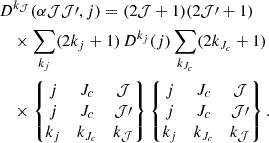8)

The total multiterm relaxation rate of the coherence (α𝒥𝒥′) is obtained by summing the partial contributions of Eq. (8) over the allowed valence-electron channels, j, of the term

$$\begin{array}{c}\hfill D^{k_{\mathcal{J}}}(\alpha \mathcal{J}\mathcal{J}\prime )={\displaystyle \sum _j}{D}^{k_{\mathcal{J}}}(\alpha \mathcal{J}\mathcal{J}\prime ,j),\end{array}$$(9)

and

$$\begin{array}{cc}& D^{k_{\mathcal{J}}}(\alpha \mathcal{J}\mathcal{J}\prime \to \alpha \mathcal{J}″\mathcal{J}\prime ″,j,j\prime )\hfill \\ \hfill & =\sqrt{(2\mathcal{J}+1)(2\mathcal{J}\prime +1)(2\mathcal{J}″+1)(2\mathcal{J}\prime ″+1)}\hfill \\ \hfill & \times {\displaystyle \sum _{k_j}}(2k_j+1)D^{k_j}(\alpha j\to \alpha j\prime ){\displaystyle \sum _{k_{J_c}}}(2k_{J_c}+1)\hfill \\ \hfill & \times \left\{\begin{array}{ccc}j& J_c& \mathcal{J}\\ j& J_c& \mathcal{J}\prime \\ k_j& k_{J_c}& k_{\mathcal{J}}\end{array}\right\}\left\{\begin{array}{ccc}j\prime & J_c& \mathcal{J}″\\ j\prime & J_c& \mathcal{J}\prime ″\\ k_j& k_{J_c}& k_{\mathcal{J}}\end{array}\right\}.\hfill \end{array}$$(10)

Here, the total multiterm transfer rate is obtained by summing over the allowed valence-electron channels for each pair, in analogy with Eq. (4) for the multilevel case and Eq. (9) for the multiterm relaxation,

$$\begin{array}{c}\hfill D^{k_{\mathcal{J}}}(\alpha \mathcal{J}\mathcal{J}\prime \to \alpha \mathcal{J}″\mathcal{J}\prime ″)={\displaystyle \sum _{\begin{array}{c}(j,j\prime )\\ j\ne j\prime \end{array}}}{D}^{k_{\mathcal{J}}}(\alpha \mathcal{J}\mathcal{J}\prime \to \alpha \mathcal{J}″\mathcal{J}\prime ″,j,j\prime ),\end{array}$$(11)

where the sum runs over all possible (j, j′) pairs with j ≠ j′; i.e., only simple-atom transfer rates D^k_j(j → j′) may enter the channel sum. We have to compute (or infer) the simple-atom rates D^k_j(j) and D^k_j(j → j′) for the valence electron to generate the full set of D^k_𝒥(α𝒥𝒥′) and D^k_𝒥(α𝒥𝒥′→α𝒥″𝒥″′) needed in the multiterm SEE.

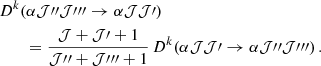
The Boltzmann factor, e^−ΔE/k_BT, can be approximated by unity, as in the case of the small fine-structure splittings of He I at T = 5000 K, where ΔE/k_BT ranges from about 1.3 × 10⁻⁵–3.1 × 10⁻⁴ within a given term. In this approach, the multiterm collisional transfer rates obey a balance relation that connects the forward (𝒥, 𝒥′) → (𝒥″, 𝒥″′) and reverse (𝒥″, 𝒥″′)→(𝒥, 𝒥′) processes through the effective pair weight, g_𝒥𝒥′ = 𝒥 + 𝒥′+1, via

$$\begin{array}{cc}& D^k(\alpha \mathcal{J}″\mathcal{J}\prime ″\to \alpha \mathcal{J}\mathcal{J}\prime )\hfill \\ \hfill & =\frac{\mathcal{J}+\mathcal{J}\prime +1}{\mathcal{J}″+\mathcal{J}\prime ″+1}{D}^k(\alpha \mathcal{J}\mathcal{J}\prime \to \alpha \mathcal{J}″\mathcal{J}\prime ″).\hfill \end{array}$$(12)

In the diagonal multilevel limit, 𝒥 = 𝒥′ and 𝒥″ = 𝒥″′, the statistical weights are reduced to 𝒥 + 𝒥′+1 = 2𝒥 + 1 and 𝒥″ + 𝒥″′ + 1 = 2𝒥″ + 1, while Eq. (12) recovers the usual multilevel detailed-balance relation for the population-transfer rates between two fine-structure levels,

$$\begin{array}{c}\hfill D^k(\alpha \mathcal{J}″\to \alpha \mathcal{J})=\frac{2\mathcal{J}+1}{2\mathcal{J}″+1}{D}^k(\alpha \mathcal{J}\to \alpha \mathcal{J}″),\end{array}$$(13)

neglecting the Boltzmann factor. This explains why only the upward (lower-energy to higher-energy) rates are listed in Tables A.2 and A.4: the downward rates follow from Eqs. (12) and (13) without further computation. We emphasize that these balance relations connect the two physically distinct processes of forward and reverse transfer; they should not be confused with a mere permutation of the indices 𝒥 ↔ 𝒥′ inside a single coherence pair, which is not a detailed-balance relation.

4. Inference of He I collisional rates from general variation laws

4.1. Cases in which the valence electron is in s-States

For s-states, the valence electron is characterized by l = 0 and, therefore, only one orbital sublevel is present. If the electron spin is neglected, isotropic collisions cannot couple different magnetic sublevels, the scattering matrix remains diagonal, and the depolarization rate of a spherically symmetric j = 1/2 level vanishes (see Derouich et al. 2005b). Depolarization can therefore arise only through spin-dependent effects. Although a j = 1/2 level cannot carry alignment, its destruction in terms of orientation remains important because it enters the recoupling expressions used to obtain depolarization and population-transfer rates in more complex atoms. In addition, it is required for interpreting polarization in hyperfine-structured levels. The appropriate treatment of these collisions is the formalism detailed in Derouich et al. (2005b, see also Derouich & Barklem 2007), which includes exchange interactions through symmetry-adapted perturbation theory based on the Murrell-Shaw-Musher-Amos formalism. Thus, the collisional physics of s-states differs fundamentally from that of p- and d-states (see the next subsection). In the present work, the depolarization and transfer rates associated with s-state contributions can therefore be computed using the variation laws of Derouich et al. (2005b).

For a simple atom in an ns  ²S_1/2 state (n is the principal quantum number), only the destruction of orientation (tensorial rank, k_j = 1) is nonzero, while population (k_j = 0) and the higher rank depolarization rates vanish. At the reference temperature, T = 5000 K, the destruction rate of orientation follows a power-law behavior with the effective principal quantum number, n^* (see Derouich et al. 2005b) via

$$\begin{array}{c}\hfill D^{k_j=1}(j=1/2,T=5000\mathrm{K})=1.0045\times {10}^{-9}{n}_{\mathrm{H}}{(n^{\ast })}^{2.979},\end{array}$$(14)

where n_H is the neutral hydrogen density in cm⁻³ and the rate is expressed in s⁻¹.

The temperature dependence of the destruction of orientation is also described by a power law (see Derouich et al. 2005b) via

$$\begin{array}{c}\hfill D^{k_j=1}(j=1/2,T)=D^{k_j=1}(j=1/2,T=5000\mathrm{K}){\left(\frac{T}{5000}\right)}^{0.416},\end{array}$$(15)

which provides an accurate description of the temperature scaling for solar and stellar atmospheric conditions.

In the present work, Eqs. (14) and (15) are used to evaluate the simple-atom destruction rate of orientation for He I levels whose valence electron occupies an s-state. For each level, the effective principal quantum number, n^*, should be determined (see Table 2 and Eq. (20) in Sect. 4.3), while the corresponding rate is computed at the required temperature. These simple-atom rates are then recoupled to the full He I fine-structure system using the angular-momentum relations described in Sect. 2.2 (the frozen-core coupling scheme) via Eqs. (3)–(6) for the multilevel rates and Eqs. (8)–(11) for the multiterm rates.

The accuracy of the He I rates associated with s-state contributions is governed by two distinct ingredients. The first is the underlying simple-atom s-state rate, namely the destruction rate of orientation computed with the spin-dependent semi-classical formalism of Derouich et al. (2005b). This part of the method explicitly includes exchange interactions through symmetry-adapted perturbation theory and has been quantitatively benchmarked: the calculated rate agrees with the fully quantum result for Na I to better than 1% at T = 5000 K, while the extension to the simple ion Ca II differs by only about 4% at the same temperature. Thus, the intrinsic uncertainty of the s-state prescription itself is small.

The second ingredient is the frozen-core reduction used to apply these simple-atom rates to He I. In this approximation, the compact inner 1s electron is kept inert, while the collision with neutral hydrogen is assumed to act predominantly on the outer active electron. Once this approximation is adopted, the recoupling to the He I fine-structure levels is purely algebraic and introduces no additional dynamical uncertainty. A direct percentage error for the frozen-core approximation in He I+H depolarizing collisions cannot yet be assigned, because no full two-electron benchmark calculation is available. Nevertheless, the present case is physically favorable: the helium core contains only one tightly bound 1s electron, unlike complex atoms or ions where the frozen core may contain many electrons or open subshells. Moreover, the broader frozen-core plus optical-electron strategy has been used successfully in depolarization and line-broadening calculations for complex systems; in the related ABO broadening theory (see Anstee 1992; Anstee & O’Mara 1991; Anstee & O’Mara 1995; Anstee et al. 1997; Barklem et al. 1998; Barklem & O’Mara 1997; Barklem et al. 1998), comparisons with solar line profiles and abundance determinations (including an agreement with meteoritic abundances), indicate typical accuracies on the order of 20% or better. Since the present s-state treatment additionally includes the spin and exchange effects absent from the standard broadening validation, the generic 20% value should be viewed as a conservative upper-bound reference, rather than as the expected uncertainty for He I. We therefore regard the present He I rates as physically reliable semiclassical estimates, with the dominant remaining uncertainty arising from the frozen-core assumption rather than from either the spin-exchange s-state rates or the angular-momentum recoupling.

4.2. Cases where the valence electron is in the p- and d-states

The collisional depolarization rates, D^k_𝒥(α𝒥), and polarization-transfer rates, D^k_𝒥, (α𝒥 → α𝒥′) required in the present work were inferred using the general variation laws established in Derouich (2020), which provide a comprehensive and unified description of (de)polarizing collisions of simple atoms with neutral hydrogen. In that work, extensive numerical calculations based on the Derouich-Sahal-Bréchot (DSB) semiclassical approach were performed for hypothetical simple atoms in p- and d-states, covering a wide range of effective principal quantum numbers, n^*. The resulting database of thousands of cross sections was then condensed into 48 analytical variation laws that express the depolarization and polarization-transfer rates as power laws of n^*.

For a given atomic level characterized by the total angular momentum, j, the tensorial order, k_j, and the effective principal quantum number, n^*, the rates at the reference temperature, T = 5000 K, are given by

$$\begin{array}{cc}\hfill D^{k_j}(j,T=5000\mathrm{K})& =n_{\mathrm{H}}\times {10}^{-9}{a}^{k_j}(j){(n^{\ast })}^{b^{k_j}(j)},\hfill \end{array}$$(16)

$$\begin{array}{cc}\hfill D^{k_j}(j\to j\prime ,T=5000\mathrm{K})& =n_{\mathrm{H}}\times {10}^{-9}{a}^{k_j}(j\to j\prime ){(n^{\ast })}^{b^{k_j}(j\to j\prime )},\hfill \end{array}$$(17)

where n_H is the hydrogen density in cm⁻³ and the coefficients a^k_j and b^k_j are tabulated in Derouich (2020).

For each fine-structure level involved in the He I atomic model, the effective principal quantum number, n^*, is first determined from the known atomic energy levels. The corresponding depolarization and polarization-transfer rates at T = 5000 K are then directly obtained by applying the above variation laws.

Given the broad thermal range of the solar chromosphere, the temperature dependence of the collisional rates must be taken into account. As discussed in Derouich et al. (2006), the (de)polarization rates due to collisions with neutral hydrogen scale with temperature as T^0.38 for p- and d-states. Therefore, the rates at an arbitrary temperature, T, can be obtained via

$$\begin{array}{cc}\hfill D^{k_j}(j,T)& =D^{k_j}(j,T=5000\mathrm{K}){\left(\frac{T}{5000}\right)}^{0.38},\hfill \end{array}$$(18)

$$\begin{array}{cc}\hfill D^{k_j}(j\to j\prime ,T)& =D^{k_j}(j\to j\prime ,T=5000\mathrm{K}){\left(\frac{T}{5000}\right)}^{0.38}.\hfill \end{array}$$(19)

This procedure allowed us to efficiently and consistently determine all the collisional depolarization, polarization-transfer, and population-transfer rates required for the multilevel and multiterm modeling of He I lines, without the need to perform new quantum or semiclassical collision calculations (Eqs. (3)–(6) and Eqs. (8)–(11)). Consequently, the He I rates benefit from the generality and robustness of the variation laws established in Derouich (2020), which were designed to be applicable to any simple atom interacting with neutral hydrogen under solar conditions.

4.3. Workflow for computing He I collisional rates

The complete procedure for computing the He I rate comprises the following steps:

1. Select the He I levels 𝒥 and 𝒥′ from the table of quantum numbers.

2. Read the corresponding quantum numbers l, s, j and L_c, S_c, J_c.

3. Read the energy, E_level, from Table 2 and compute n^* using

   $$\begin{array}{c}\hfill n^{\ast }=\frac{1}{\sqrt{2(E_{\text{ionization}}-E_{\text{level}})}}\end{array}$$(20)

   where, for the He I atom, E_ionization = 0.9035699 a.u. relative to the ground-state energy.

4. Evaluate the simple-atom rates via

   • the Derouich (2020) variation-law equations (Eqs. (16)–(19)) for p- and d-states;

   • the Derouich et al. (2005b) equations (Eqs. (14) and (15)) for s-states.

5. Insert the simple-atom rates into the transfer and depolarization rate equations (Eqs. (3)–(6) for the multilevel formulation, or Eqs. (8)–(11) for the multiterm formulation).

6. Perform the linear combination of 9j-symbol summations to obtain all rates for the atomic model of He I. The transfer rates are computed by retaining only off-diagonal valence-electron channels with j ≠ j′. The depolarization rates are computed from the corresponding simple-atom depolarization channels and then summed over the allowed j contributions.

This procedure provides a consistent and computationally efficient way to construct the full set of He I collisional rates needed for the SEE and polarized radiative-transfer calculations. The resulting multilevel depolarization rates and multilevel population- and polarization-transfer rates are listed in Tables A.1 and A.2, respectively. The multiterm depolarization coefficients and multiterm transfer rates are listed in Tables A.3 and A.4, respectively.

It is useful to note that if 𝒥 ≠ 𝒥 ′, the value k_𝒥 = 0 is not allowed by the angular-momentum condition,

$$|\mathcal{J}-\mathcal{J}\prime |\le k_{\mathcal{J}}\le \mathcal{J}+\mathcal{J}\prime .$$

Therefore, $D^0(\alpha \mathcal{J}\mathcal{J}\prime )=0$ for 𝒥 ≠ 𝒥 ′. For this reason, only the nonzero even tensorial ranks, k_𝒥 > 0, are listed for the relaxation, rates $D^{k_{\mathcal{J}}}(\alpha \mathcal{J}{\mathcal{J}}^{\prime })$. In contrast, the rank k_𝒥 = 0 transfer rates are nonzero overall; in fact, the rank k_𝒥 = 0 is allowed for diagonal pairs $(\mathcal{J},\mathcal{J})$ and $(\mathcal{J}″,\mathcal{J}″)$, but it is not allowed for off-diagonal coherences with 𝒥 ≠ 𝒥 ′ and/or 𝒥 ″ ≠ 𝒥 ′″.

5. Conclusion

We present a new set of collisional depolarization, polarization-transfer, and population-transfer rates applicable to isotropic collisions with neutral hydrogen, for the singlet and triplet terms of neutral helium that control the main solar He I diagnostics, including the 10830 Å and D₃ multiplets. These rates have been computed in both the multilevel and multiterm formulations; the extended tables are given in Appendix A for T = 5000 K, together with the relevant scaling laws for chromospheric and prominence temperatures. These results address an important missing ingredient in the modeling of He I spectropolarimetry. The 10830 Å and 5876 Å lines are among the most sensitive probes of magnetic fields in the upper solar atmosphere, where their polarization is shaped by atomic-level polarization, the Hanle effect, and the Zeeman effect. Forward-modeling and inversion numerical codes allow for the multilevel or multiterm SEE to be computed for the He I density matrix. The rates given here can therefore be incorporated directly, replacing the order-of-magnitude estimates commonly adopted so far.

Our results provide a quantitative basis for reassessing the role of neutral-hydrogen collisions in destroying or transferring atomic polarization. In particular, it is now possible to test the assumption usually adopted in solar physics that collisional depolarization is generally expected to be negligible, especially in typical quiescent prominences because the required hydrogen densities are too high. At the same time, our tabulated rates allow us to identify denser regimes, such as active-region filaments, dense spicules, post-flare loops, and coronal rain, where collisional depolarization rates may become comparable to radiative rates. They also separate the effects of transfer rates from depolarization rates, which are often merged in simplified treatments.

Acknowledgments

This research work was funded by Institutional Fund Projects under grant no. (IFPIP:1001-130-1443). The authors gratefully acknowledge technical and financial support provided by the Ministry of Education and King Abdulaziz University, DSR, Jeddah, Saudi Arabia

References

Appendix A: Additional collisional rate tables

This appendix provides the additional collisional rate tables for the multilevel and multiterm formulations.

All Tables

References

- Anan, T., Schad, T. A., Kitai, R., et al. 2021, ApJ, 921, 39 [NASA ADS] [CrossRef] [Google Scholar]
- Anstee, S. D. 1992, Ph.D. Thesis, University of Queensland, Australia [Google Scholar]
- Anstee, S. D., & O’Mara, B. J. 1991, MNRAS, 253, 549 [NASA ADS] [CrossRef] [Google Scholar]
- Anstee, S. D., & O’Mara, B. J. 1995, MNRAS, 276, 859 [Google Scholar]
- Anstee, S. D., O’Mara, B. J., & Ross, J. E. 1997, MNRAS, 284, 202 [CrossRef] [Google Scholar]
- Asensio Ramos, A., Trujillo Bueno, J., & Landi Degl’Innocenti, E. 2008, ApJ, 683, 542 [Google Scholar]
- Barklem, P. S. 1998, Ph.D. Thesis, University of Queensland, Australia [Google Scholar]
- Barklem, P. S., & O’Mara, B. J. 1997, MNRAS, 290, 102 [Google Scholar]
- Barklem, P. S., O’Mara, B. J., & Ross, J. E. 1998, MNRAS, 296, 1057 [Google Scholar]
- Blum, K. 1981, Density Matrix Theory and Applications (New York: Plenum Press) [Google Scholar]
- Bommier, V., & Sahal-Bréchot, S. 1978, A&A, 69, 57 [Google Scholar]
- Casini, R., López Ariste, A., Tomczyk, S., & Lites, B. W. 2003, ApJ, 598, L67 [Google Scholar]
- Centeno, R., Trujillo Bueno, J., & Asensio Ramos, A. 2010, ApJ, 708, 1579 [NASA ADS] [CrossRef] [Google Scholar]
- de la Cruz Rodríguez, J., & Leenaarts, J. 2024, A&A, 685, A85 [NASA ADS] [CrossRef] [EDP Sciences] [Google Scholar]
- Derouich, M. 2020, ApJS, 247, 72 [NASA ADS] [CrossRef] [Google Scholar]
- Derouich, M., & Barklem, P. S. 2007, A&A, 462, 1171 [NASA ADS] [CrossRef] [EDP Sciences] [Google Scholar]
- Derouich, M., & Qutub, S. 2024, A&A, 683, A173 [NASA ADS] [CrossRef] [EDP Sciences] [Google Scholar]
- Derouich, M., Sahal-Bréchot, S., Barklem, P. S., & O’Mara, B. J. 2003a, A&A, 404, 763 [NASA ADS] [CrossRef] [EDP Sciences] [Google Scholar]
- Derouich, M., Sahal-Bréchot, S., & Barklem, P. S. 2003b, A&A, 409, 369 [NASA ADS] [CrossRef] [EDP Sciences] [Google Scholar]
- Derouich, M., Sahal-Bréchot, S., & Barklem, P. S. 2004a, A&A, 414, 373 [NASA ADS] [CrossRef] [EDP Sciences] [Google Scholar]
- Derouich, M., Sahal-Bréchot, S., & Barklem, P. S. 2004b, A&A, 426, 707 [NASA ADS] [CrossRef] [EDP Sciences] [Google Scholar]
- Derouich, M., Sahal-Bréchot, S., & Barklem, P. S. 2005a, A&A, 434, 779 [NASA ADS] [CrossRef] [EDP Sciences] [Google Scholar]
- Derouich, M., Barklem, P. S., & Sahal-Bréchot, S. 2005b, A&A, 441, 395 [NASA ADS] [CrossRef] [EDP Sciences] [Google Scholar]
- Derouich, M., Bommier, V., Malherbe, J. M., & Landi Degl’Innocenti, E. 2006, A&A, 457, 1047 [NASA ADS] [CrossRef] [EDP Sciences] [Google Scholar]
- Díaz Baso, C. J., Martínez González, M. J., & Asensio Ramos, A. 2019, A&A, 625, A128 [NASA ADS] [CrossRef] [EDP Sciences] [Google Scholar]
- Esteban Pozuelo, S., Asensio Ramos, A., Trujillo Bueno, J., et al. 2025, A&A, 696, A109 [NASA ADS] [CrossRef] [EDP Sciences] [Google Scholar]
- Hanle, W. 1924, Z. Phys., 30, 93 [NASA ADS] [CrossRef] [Google Scholar]
- Kramida, A., Ralchenko, Yu., & Reader, J.& NIST ASD Team. 2022, NIST Atomic Spectra Database (ver. 5.10) (Gaithersburg, MD: National Institute of Standards and Technology), https://doi.org/10.18434/T4W30F [Google Scholar]
- Kuckein, C., Centeno, R., Martínez Pillet, V., et al. 2009, A&A, 501, 1113 [NASA ADS] [CrossRef] [EDP Sciences] [Google Scholar]
- Kuckein, C., González Manrique, S. J., Sobotka, M., et al. 2020, A&A, 640, A71 [NASA ADS] [CrossRef] [EDP Sciences] [Google Scholar]
- Landi Degl’Innocenti, E. 1982, SoPh, 79, 291 [Google Scholar]
- Landi Degl’Innocenti, E., & Landolfi, M. 2004, Polarization in Spectral Lines (Dordrecht: Kluwer Academic Publishers), Astrophys. Space Sci. Lib., 307 [Google Scholar]
- Leenaarts, J., van Noort, M., de la Cruz Rodríguez, J., et al. 2025, A&A, 696, A3 [NASA ADS] [CrossRef] [EDP Sciences] [Google Scholar]
- López Ariste, A., & Casini, R. 2002, ApJ, 575, 529 [Google Scholar]
- Merenda, L., Trujillo Bueno, J., Landi Degl’Innocenti, E., & Collados, M. 2006, ApJ, 642, 554 [Google Scholar]
- Nienhuis, G. 1976, J. Phys. B: At. Mol. Phys., 9, 167 [Google Scholar]
- Omont, A. 1977, Prog. Quantum Electron., 5, 69 [Google Scholar]
- Orozco Suárez, D., Asensio Ramos, A., & Trujillo Bueno, J. 2014, A&A, 566, A46 [NASA ADS] [CrossRef] [EDP Sciences] [Google Scholar]
- Quintero Noda, C., Schlichenmaier, R., Bellot Rubio, L. R., et al. 2022, A&A, 666, A21 [NASA ADS] [CrossRef] [EDP Sciences] [Google Scholar]
- Rimmele, T. R., Warner, M., Keil, S. L., et al. 2020, SoPh, 295, 172 [Google Scholar]
- Sahal-Bréchot, S. 1977, ApJ, 213, 887 [Google Scholar]
- Sahal-Bréchot, S., Derouich, M., Bommier, V., & Barklem, P. S. 2007, A&A, 465, 667 [NASA ADS] [CrossRef] [EDP Sciences] [Google Scholar]
- Sasso, C., Lagg, A., & Solanki, S. K. 2011, A&A, 526, A42 [NASA ADS] [CrossRef] [EDP Sciences] [Google Scholar]
- Schad, T. A., Penn, M. J., Lin, H., & Judge, P. G. 2016, ApJ, 833, 5 [Google Scholar]
- Stenflo, J. O. 1994, Solar Magnetic Fields (Dordrecht: Kluwer Academic Publishers) [Google Scholar]
- Trujillo Bueno, J., & del Pino Alemán, T. 2022, Annu. Rev. Astron. Astrophys., 60, 415 [Google Scholar]
- Trujillo Bueno, J., Landi Degl’Innocenti, E., Collados, M., Merenda, L., & Manso Sainz, R. 2002, Nature, 415, 403 [Google Scholar]
- Trujillo Bueno, J., Merenda, L., Centeno, R., Collados, M., & Landi Degl’Innocenti, E. 2005, ApJ, 619, L191 [NASA ADS] [CrossRef] [Google Scholar]
- Vicente Arévalo, A., Štěpán, J., del Pino Alemán, T., & Martínez González, M. J. 2023, A&A, 675, A45 [NASA ADS] [CrossRef] [EDP Sciences] [Google Scholar]
- Wiegelmann, T., Thalmann, J. K., & Solanki, S. K. 2014, A&A Rev., 22, 78 [Google Scholar]