


| Issue |
A&A
Volume 711, July 2026
|
|
|---|---|---|
| Article Number | A280 | |
| Number of page(s) | 10 | |
| Section | Astrophysical processes | |
| DOI | https://doi.org/10.1051/0004-6361/202660654 | |
| Published online | 23 July 2026 | |
Iron He-triplet signatures of shocks in the hottest galaxy clusters
Z/W line ratio, line broadening, and electron-ion temperature equilibration
1
Max Planck Institute for Astrophysics, Karl-Schwarzschild-Str. 1, D-85741 Garching, Germany
2
Department of Astronomy, University of Maryland, College Park, MD 20742, USA
3
X-ray Astrophysics Laboratory, NASA Goddard Space Flight Center, Greenbelt, MD 20771, USA
4
Center for Research and Exploration in Space Science and Technology, NASA Goddard Space Flight Center, Greenbelt, MD 20771, USA
5
Rudolf Peierls Centre for Theoretical Physics, Department of Physics, University of Oxford, Clarendon Laboratory, Parks Rd, Oxford OX1 3PU, UK
6
Center for Astrophysics | Harvard & Smithsonian, 60 Garden St., Cambridge, MA 02138, USA
7
Department of Astronomy & Astrophysics, University of Chicago, Chicago, IL 60637, USA
8
Leiden Observatory, Leiden University, PO Box 9513, 2300 RA, Leiden, The Netherlands
9
Department of Theoretical Physics and Astrophysics, Masaryk University, Brno 61137, Czechia
★ Corresponding author: This email address is being protected from spambots. You need JavaScript enabled to view it.
Received:
28
April
2026
Accepted:
8
June
2026
Abstract
A merger of clusters naturally drives shocks with Mach number ℳ ≲ 3 in the intracluster medium (ICM). This process creates several distinct signatures, including sharp surface-brightness “edges”, temperature, and gas-velocity jumps. The low density of the ICM implies that ionization balance and electron-ion equilibration timescales can be long enough to produce additional observable signatures. Here, we focus on two “transient” spectral signatures accessible with high-energy-resolution telescopes such as XRISM, even in unfavorable geometries, for example when we are looking inside the Mach cone of the shock, which precludes the appearance of sharp edges in X-ray images. In this work, we focus on (i) the Z/W line ratio of the Fe XXV triplet and (ii) the contribution of ions with Ti > Te to the line width, which might be mistakenly interpreted as gas turbulence. We demonstrate that the Z/W ratio can serve as a proxy for the nonequilibrium state of the shocked ICM and facilitate interpretation of the line broadening. We conclude that these spectral signatures are within reach of missions such as XRISM and can be used to constrain the electron heating at collisionless cluster shocks, as well as the rate of subsequent temperature equilibration between different particle species.
Key words: atomic processes / line: formation / line: profiles / shock waves / galaxies: clusters: intracluster medium
© The Authors 2026
 Open Access article, published by EDP Sciences, under the terms of the Creative Commons Attribution License (https://creativecommons.org/licenses/by/4.0), which permits unrestricted use, distribution, and reproduction in any medium, provided the original work is properly cited.
This article is published in open access under the Subscribe to Open model.
Open access funding provided by Max Planck Society.
1. Introduction
Cluster mergers are common in cosmological simulations and observations. Minor mergers, in which one of the merging clusters is much less massive than the other, are very frequent, whereas equal-mass mergers are rarer. The latter often lead to spectacular features that reveal the physics of the merger process (see e.g. Markevitch & Vikhlinin 2007, for a review). The ICM temperature in galaxy clusters scales with the mass as TX ∝ GMv/Rv ∼ Vv2, where the subscript “v” denotes characteristic virial quantities. Since the sound speed and the virial velocity follow the same scaling with mass, one expects a similar range of shock Mach numbers, independent of the cluster mass. For a Navarro-Frenk-White potential with a concentration parameter of c ∼ 2 − 6 (e.g., Comerford & Natarajan 2007), the velocity of a point mass on a parabolic trajectory reaches ∼3.05 − 3.3Vv in the cluster center. This sets a natural characteristic value for the maximal Mach number, ℳ ≲ 3, expected during pericenter passage. We discuss a generic case throughout the text, with examples such as the Bullet cluster (Markevitch et al. 2002) and the Peanut cluster (Lyskova et al. 2025) in mind. For illustration, we assume an initial gas temperature of 7 keV (for Mv ∼ 1015 M⊙) and a shock with ℳ = 3.2.
In the context of cluster shocks, the ICM density can be very low (ne ∼ 10−3 − 10−4 cm−3), implying that the relaxation timescales can be on the order of 108 yr, and departures from ionization equilibrium or different temperatures of electrons and ions might persist long enough to produce observable signatures (e.g., Fox & Loeb 1997; Chièze et al. 1998; Takizawa 1999; Markevitch & Vikhlinin 2007; Wong & Sarazin 2009; Akahori & Yoshikawa 2010; Russell et al. 2012; Di Mascolo et al. 2019; Sarkar et al. 2024; Norseth et al. 2025). A similar set of processes defines the properties of heated plasma in supernova-remnant shocks in the interstellar medium (ISM) (e.g., Bykov et al. 2008; Vink 2012; Raymond et al. 2023). However, unlike the ISM, the ICM is hot, except in the very outskirts, and the sonic Mach number ℳ is typically not much larger than three. Another difference is that most of the ICM has plasma 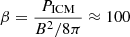 , where PICM is the ICM thermal pressure and B is the magnetic field; therefore, the Alfven Mach number is larger, ℳA = β1/2ℳ ∼ 10ℳ.
The He-like triplet diagnostic is one of the powerful probes of low-density hot collision-dominated plasma (e.g., Porquet et al. 2001). The most prominent lines are normally the well-separated resonance W (1s21S0 – 1s2p1P1) line and the forbidden magnetic-dipole Z (1s21S0 – 1s2s3S1) line, while the intercombination Y (1s21S0 – 1s2p3P1) and magnetic-quadrupole X (1s21S0 – 1s2p3P2) lines are often blended by dielectronic satellites. The non-equilibrium ionization (NEI) signatures associated with the He-like triplet of high-Z elements have long been considered in the literature (e.g., Mewe & Schrijver 1978; Liedahl 1999; Oelgoetz & Pradhan 2004). Here, we discuss these effects for an idealized case of a plane-parallel shock in the ICM, bearing in mind the capabilities of X-ray calorimeters such as the XRISM observatory (Tashiro et al. 2025), to complement merger signatures with high-resolution spectroscopic information.
We consider two models in the next section.
The first model assumes that the downstream temperatures of all species are equal immediately after the shock, and only the ionization balance evolves with time. A parameter τ = net ∼ 1012 cm−3 s, where ne is the electron density, sets the characteristic timescale t for NEI effects in this model, in particular, deviations of the relative line strengths from the collisional ionization equilibrium (CIE) predictions for the electron temperature measured from the shape of the continuum spectrum.
In the second model, the electrons and ions have different temperatures downstream of the shock and gradually equilibrate via Coulomb collisions. In this model,
-
electrons are heated adiabatically, while ions undergo adiabatic heating and are additionally heated in proportion to their mass. Beyond the NEI effects, line widths are then governed by the different ion temperatures;
-
ions first equilibrate with each other, lowering their temperatures to the proton temperature on a timescale similar to that of ionization equilibrium;
-
electrons equilibrate with protons (and other ions) on a timescale approximately ten times longer than ion-proton equilibration, with the ionization equilibrium evolving along with the electron temperature, while the thermal broadening of ions follows the proton temperature.
2. Model
2.1. Relevant physical processes
As an illustrative example, we consider a hot plasma with an initial temperature T0 = 7 keV. In the initial state, the electron and ion temperatures are equal (Te = Ti), and the plasma is in the state of CIE corresponding to this temperature1. The plasma is optically thin, and the level population corresponds to the coronal approximation. A plane-parallel collisionless shock with ℳ = 3.2 instantly changes the density and the mean plasma temperature according to the Rankine-Hugoniot conditions for the adiabatic index γ = 5/3. For ℳ = 3.2, the density and temperature jumps are ρds ≈ 3.09ρ0 and Tds ≈ 4.06T0, with the subscript “ds” denoting downstream of the shock.
2.2. Electron-ion temperature equilibration
For the downstream temperatures of different species, we consider two cases:
-
A: Te = Tp = TZ = Tds for all species.
-
B: Te ≠ Tp ≠ TZ and pure Coulomb collisions control the temperature equilibration.
In the second case, we set the initial temperatures to be “maximally different”. Namely, we assume that ion temperatures, in addition to adiabatic heating, scale with the ion masses Ti ∝ mi, while the initial electron temperature corresponds to the adiabatic compression set by the density jump, such that Te,ds = T0(ρds/ρ0)(γ−1) ≈ 2.12 T0 (for a compression ratio of 3.09). This assumption corresponds to the limit in which each particle species thermalizes a fraction of the shock speed independently, without any energy exchange between particle species. It may occur in collisionless shocks, where the shock transition is mediated by plasma turbulence and electromagnetic fields instead of collisions between particles (see, e.g. Ghavamian et al. 2007; Bykov et al. 2008; Vink et al. 2015; Raymond et al. 2017, and references therein). With this definition, electrons, protons, and Fe XXV ions have the following temperatures immediately downstream: Te,ds ≈ 15 keV, Tp,ds ≈ 43 keV, and TFe,ds ≈ 1.5 MeV, respectively. Unlike high-Mach-number shocks in young supernova remnants (Ghavamian et al. 2013; Raymond et al. 2023), where the Te,ds/Tp,ds ratio can be very low (under the same assumptions), in clusters this ratio is modest by virtue of the limited sonic Mach number, so that the adiabatically heated electrons are only a factor of ≲3 colder than protons. The adiabatic heating of electrons at ICM shocks is also supported by observations (e.g., Russell et al. 2022; Sarkar et al. 2024; Norseth et al. 2025).
Subsequent evolution of the temperatures in case B can be reasonably accurately described by coupling between electrons and protons, and between ions and protons, namely
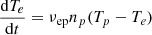 (1)
(1)
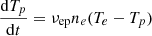 (2)
(2)
 (3)
(3)
where ne, np, and nZ are the number densities of electrons, protons, and heavy ions, respectively; the νab terms define the rates of energy exchange between two species, a and b (Spitzer 1962). A more accurate treatment would include helium and coupling between all species. We show this in Appendix C. However, for our illustrative example, the three equations above are sufficient. The first two describe the energy exchange between electrons and protons. Heavy ions are not important in the overall energy budget due to their low abundance. Therefore, we can trace their temperature evolution through collisions with electrons and protons (the third equation), but we can ignore their back-reaction on other species. Since we ignore the impact of He, it would be logical to ignore the first term on the right-hand side of the third equation, which is subdominant compared to the rate of energy exchange between iron and helium ions. We keep it to maintain a self-consistent approximation in which all ions heavier than a proton (by assumption) make a negligible contribution to the total energy density. As we illustrate in Appendix C, this is sufficient for typical applications, unless very accurate predictions are required.
The evolution of Te, Tp, and TZ in our illustrative model is shown in Fig. 1. As expected, for pure Coulomb collisions, TZ approaches Tp on a timescale tZ, p, which is an order of magnitude shorter than that of the electron-ion equilibration. The corresponding value of τZ, p = tZ, pne ≈ tZ, pnp ≲ 1012 cm−3 s, while τe, p ∼ 1013 cm−3 s. As shown in the following (Sect. 2.3), the typical value of τCIE required to establish the ionization equilibrium is on the same order as τZ, p and is smaller than τe, p. This implies that for τ ≳ 1012 cm−3 s, the ion fractions are close to CIE and follow the Te(t) evolution. The observed spectra (for these values of τ) can therefore be represented as a superposition of CIE spectra with different plasma temperatures. However, the thermal line width of the ions is set by TZ, which can be larger than Te up to τ ∼ 1013 cm−3 s. Therefore, the measured line width may be erroneously attributed to turbulence if only iron lines are observed (at least two elements with different masses are required to differentiate turbulence from thermal broadening). We return to this issue in Sect. 3.2.
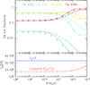 |
Fig. 1. Coulomb-collision-mediated temperature equilibration between electrons, protons, and He-like iron ions (Fe XXV) in the limit of adiabatic heating of electrons at the shock. The Fe XXV ions temperature, TZ, approaches Tp at τ ∼ 1012 cm−3 s and then evolves together with Tp. The NEI timescale (see Fig. 2 below) is approximately the same as the TZ ≫ Tp timescale. Ions remain hotter than electrons up to τ ∼ 2 − 3 × 1013 cm−3 s. Therefore, the Fe XXV ions are hotter than Te up to this value of τ, and the thermal broadening of the Fe XXV lines is larger than that predicted from the electron temperature Te derived from the continuum shape. The helium abundance is set to zero for this plot (see Fig. C.1 for the impact of helium). |
We note that Coulomb collisionality is unlikely to govern all equilibration processes in the ICM. Magnetic fields can effectively increase the rate of ion-electron collisions via scattering from plasma instabilities (Schekochihin & Cowley 2006) or anisotropic transport along field lines (Kunz et al. 2011). A reduced effective viscosity below the Coulomb level has been detected in the ICM via the suppression of Kelvin-Helmholtz instabilities in cold fronts (e.g., Markevitch & Vikhlinin 2007; Zuhone & Roediger 2016) and via the extension of density fluctuations power spectra into the viscous regime (Zhuravleva et al. 2019; Heinrich et al. 2024). Thus, the actual isotropisation rate is likely to lie somewhere between cases A and B. However, this does not necessarily mean that the temperature equilibration rate is also enhanced, since the latter requires the transfer of energy from heavier to lighter particles (from ions to electrons) rather than the randomization of particle velocities and momentum exchange.
2.3. NEI and the He-like triplet
To study the time-varying ionization balance and line intensities, we used two collisional-radiative models, namely, the CHIANTI database (Dere 2007; Del Zanna et al. 2021) and the NOMAD code (Ralchenko & Maron 2001; see Appendix for more details). As shown in the following, good agreement between two independent sets of simulations provides extra confidence in the derived results.
The top panel of Fig. 2 shows the time evolution of the iron ion fractions (Fe XXIV–XXVII). The solid lines (CHIANTI) and open squares (NOMAD) correspond to the case Te = Ti, while the dashed lines illustrate the case in which the electron temperature evolves in time due to Coulomb collisions.
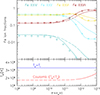 |
Fig. 2. Ionization balance and temperature evolution in the shocked medium. Bottom: Evolution of Te. The solid blue line corresponds to the Te = Ti = const case, while the dashed red line shows the “Coulomb” temperature equilibration, with Te initially set by adiabatic compression in the ℳ = 3.2 shock. In this case, Te rises slowly and does not reach Tp even at τ = 1012 cm−3 s. Top: Evolution of ionization balance. Solid lines show the Te = Ti case, based on CHIANTI rates, and open squares show the NOMAD results. Dashed lines show the ion fraction evolution when the electron temperature itself evolves with time, as shown in the bottom panel. |
The impact of nonequilibrium ionization on the line ratios has long been recognized (e.g., Mewe & Schrijver 1978; Liedahl 1999), in particular for conditions relevant to solar flares and laboratory plasmas. In these studies, the initial temperatures were typically low, and Li-like ions played a particularly important role once the temperature increased suddenly, driving the Z/W flux ratio above the characteristic CIE values. In contrast, in massive, high-temperature clusters, the fraction of Li-like iron ions is lower in the initial state, and the increased rate of inner-shell ionizations of these ions (contributing to the Z line) remains subdominant to the increased rate of Fe XXV collisional excitations populating the W line. Table B.1 lists the key properties of the Fe XXV triplet and Fe XXVI Lyα doublet lines.
Fig. 3 illustrates the impact of the instantaneous change in electron temperature from T0 to T1 on the Z/W line intensity ratio. In this regime, the ionization balance corresponds to CIE at temperature T0, while the electron temperature is T1. The top-left corner corresponds to T1 > T0 scenario, e.g., a shock, while the bottom-right corresponds to the T1 < T0 case, e.g., fast expansion. The former regime leads to a decrease in the Z/W ratio, while the latter pushes the ratio in the opposite direction.
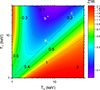 |
Fig. 3. Simulated Z/W line intensity ratio (colors; NOMAD simulation) for an instantaneous change in electron temperature from T0 to T1 in the limit of small τ. Locations a and c correspond to the flux ratios for the initial and final states with T = 7 keV and T = 28 keV, respectively. The dashed diagonal line shows the locus of other equilibrium states with T1 = T0. Location b corresponds to the intermediate case with T0 = 7 keV, T1 = 28 keV, and τ = 1010 cm−3 s. A similar ratio is expected over a wide range of τ ≲ 3 × 1010 cm−3 s. This transient state with an anomalously low Z/W ratio may serve as a signature of freshly shocked hot NEI plasma. |
Fig. 4 shows the evolution of the Z/W flux ratio as a function of the ionization parameter τ for our fiducial model. We produced the ratios with NOMAD following the procedure described in the Appendix. As explained therein, during the NEI “frozen ionization balance phase” at τ ≲ 1010 s/cm3 the Z/W flux ratio is governed by several factors, such as ion populations and modified rate coefficients for electron-impact processes.
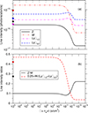 |
Fig. 4. Time-dependent (a) line intensities and (b) line intensity ratios for He- and H-like Fe from the NOMAD simulation (T0 = 7 keV, T1 = 28 keV, Te = Tp case). The 0.25 scaling factor applied to the W/Lyα ratio places all data on the same scale. Solid circles show the corresponding values at τ = 0, i.e., T0 = 7 keV. |
2.4. He-like versus H-like
Another useful and currently accessible diagnostic is the ratio of the Fe XXVI Lyα and Fe XXV triplet fluxes. Under CIE conditions, this ratio serves as a line-based temperature proxy. Studies have also considered the NEI aspects of this flux ratio (e.g., Prokhorov 2010; Inoue et al. 2016). For our baseline model with a rather hot ICM, the Boltzmann factor (e−ΔE/kT) is already close to unity (ΔE ≪ kT), and the flux ratio is mostly driven by changes in the iron ionization fractions, from the He-dominated state at the beginning to the H-dominated state at large τ. This is illustrated by dashed lines in Fig. 4. Fig. 5 shows a comparison of the line ratios for the Te = Ti and evolving Te cases. This figure also illustrates the impact of the shock strength (Mach numbers of 3.2 and 1.8) on the magnitude of the effect. Qualitatively, suppression of the Z/W ratio is always present, although a factor of three decreases requires a shock with ℳ ≳ 3.
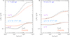 |
Fig. 5. Left: Evolution of Z/W (solid lines) and Ly/W (dashed lines) ratios following an instantaneous (black) and Coulomb-collisions-mediated (red) increase in electron temperature from 7 to 28 keV (corresponding to ℳ = 3.2 shock). The dashed blue line shows the ratio for a kT = 7 keV CIE plasma. Right: Same as in the left panel but for an initial temperature of 6.5 keV and a final temperature of 12 keV (corresponding to a ℳ = 1.8 shock). While the Z/W flux ratio differs between the Te = Tp and Te < Tp cases, it remains lower than the CIE-predicted values. The evolution of the Ly/W ratio is driven primarily by time-dependent changes in the ionization balance. |
The key role of NEI effects in the Lyα/W ratio is that, due to time-dependent changes in the ionization fractions, this ratio can take different values for the same electron temperature derived from the continuum shape. This provides additional flexibility in describing spectra in merging clusters and can itself serve as evidence for recently shocked gas in the system.
We note in passing that none of the nonstationary effects considered in this study directly affects the ratio of the Lyα doublet components in Fe XXVI. In the NOMAD calculations, this ratio (Lyα3/2/Lyα1/2) is 1.94 (or 1.8 if a contribution of 1s–2s M1 transitions is taken into account) and is about the same upstream and downstream of the shock. Therefore, the anomalies reported in XRISM Collaboration (2025) remain unexplained. Finite (and different) optical depths of the two components can modify the flux ratio, suppressing more the Lyα3/2 if the scattering “screen” lies between the bright core and the observer (see examples in Churazov et al. 2010). In particular, a configuration with a velocity offset of ∼900 km s−1 between the emitting and scattering materials might result in the red-shifted Lyα3/2 line falling in resonance with the Lyα1/2 transition and undergoing stronger scattering (as in the case considered in Khabibullin & Sazonov 2012). However, the estimated Coma optical depth in these lines is small (e.g., Sazonov et al. 2002) and does not resolve the anomaly (XRISM Collaboration 2025). We also note that, given sufficiently high photon-count statistics, the ratio of the Fe XXV Kβ to Fe XXV Kα − W line can be used to estimate possible suppression of the resonant component, since this ratio is virtually insensitive to the ionization state and electron temperature of the plasma when kTe ≫ EKβ − EW ≈ 1 keV.
2.5. Line broadening
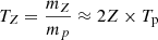
The broadening of the Fe XXV and Fe XXVI lines is a direct proxy of ion motions. It can be subdivided into thermal motions of individual ions and macroscopic plasma motions. Since the thermal velocity scales as  , where mZ ≈ 2Zmp is the ion mass, the contribution of thermal motions to the line width is the smallest for heavy ions, which therefore provides the best constraints on the ICM velocities. Most often, CIE conditions are assumed and TZ = Te. This allows the temperature to be constrained from the broad-band X-ray spectrum and the line ratios, predicts pure thermal broadening, and determines the additional velocity broadening needed to describe the observed line width. However, these assumptions may not be valid downstream of the shock. As shown in Fig. 1, the temperature of iron ions can be higher than the electron temperature for τ ≲ 1013 cm−3 s, while for τ ≲ 1011 cm−3 s, even the CIE assumption is not valid. Figure 6 illustrates these cases for our fiducial model with pure Coulomb collisions and no plasma bulk motions. In reality, supersonic bulk motions contributing to the observed line width must be present in the shock scenario unless the normal to the shock front lies exactly in the plane of the sky. Essentially, the excess line broadening (e.g., in the TZ ∝ mZTp scenario) results from isotropisation of the ion velocity jump at the shock front. Therefore, correct interpretation of the observed line broadening requires knowledge of the flow geometry.
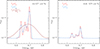 |
Fig. 6. Triplet spectrum for different assumptions about the ion temperature and different ionization parameter τ. Left: Case with τ = 1011 cm−3 s. The red, blue, and brown curves show TZ = Te, TZ = Tp, and |
3. Discussion
3.1. Nonequilibrium versus equilibrium emission measure
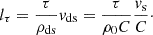
We first performed an order-of-magnitude comparison of the contribution of shocked gas to X-ray spectra with that of unshocked gas. Specifically, we are interested in regions with a characteristic ionization parameter τ comparable either to the NEI scale or to the Te ≠ Tp scale. We considered a planer shock viewed along the normal to the shock front. The downstream density and velocity are ρds = Cρ0 and vds = vs/C, where C is the compression factor. The length lτ of the downstream region with the ionization parameter smaller than τ is
 (4)
(4)
Therefore, the line-of-sight-integrated emission measure of this region is
 (5)
(5)
This value can be compared with the cluster emission measure along the line of sight,
 (6)
(6)
where Rcl is the characteristic size of the region that dominates X-ray emission. Thus, the ratio
 (7)
(7)
determines the relative contributions of the nonequilibrium part of the shock-heated gas to the total cluster flux. For a typical cluster density profile, the distance from the cluster center r can be used as Rcl. Furthermore, the quantity ρ0Rcl ∼ ρ(r)r indicates where in the cluster the impact of the shock is expected to be strongest. This is illustrated in Fig. 7. There, we set vs = vr, the velocity of a particle on a parabolic orbit in the NFW potential. We also set ρ(r) to the mean density profile of the simulated clusters from O’Neil et al. (2021). Observationally, finding examples of clusters in which the shock crosses the center is challenging, since this phase is short-lived (see, however, Lyskova et al. 2025, for examples of merging clusters close to the pericenter passage). It is also difficult to obtain detailed spectra from cluster outskirts with the current generation of X-ray telescopes due to the very low gas density and hence low flux. Therefore, the most promising are the intermediate regions within R500c. As is clear from Fig. 7, the contribution of the shock-heated gas at these radii is ∼10% for τ ≲ 1011 cm−3 s and of order unity for τ ≲ 1012 cm−3 s. Compared with Fig. 1, we conclude that under favorable conditions the contribution of the shock can be large enough to produce observable spectral signatures associated with the ionization parameter τ ∼ 1011 cm−3 s.
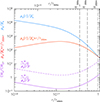 |
Fig. 7. Emission measure EMτ of shocked gas with the ionization parameter τ below a given threshold, relative to the emission measure EMcl of unshocked gas at the same distance from the cluster center (see Eq. 7). The solid and dashed purple lines show the ratio EMτ/EMcl for τ = 1011 and 1012 cm−3 s, respectively. For the shock velocity, we use the velocity vr of a point mass on a parabolic orbit. The blue and red lines show the overdensity of baryons as a function of radius and the product of overdensity and radius, respectively. The reciprocal of the latter quantity is the key quantity that determines the ratio EMτ/EMcl. The plots show that regions with τ ∼ 1011 cm−3 s can contribute ∼10% to the line-of-sight emission measure, while for τ ∼ 1012 cm−3 s the contributions from shocked and unshocked regions can be comparable. This conclusion holds for essentially any projected distance from the cluster center, although projection effects may also play a role. |
3.2. Diagnostic
The baseline spectral model used to describe emission from galaxy clusters is the optically thin thermal plasma emission model in CIE. The second commonly used model is a two-temperature CIE model that accounts for plasma with different temperatures observed along the same line of sight. The features associated with deviations from the ionization or electron-ion temperature equilibria might not be adequately captured by the two-temperature model. As discussed in Sect. 2, there are two characteristic values of τ, which are associated with specific nonequilibrium features in the X-ray spectra. Namely,
-
For τ ≲ 1012 cm−3 s, the Z/W ratio in the Fe XXV triplet can be anomalously low due to NEI effects (see Fig. 3).
-
For τ ≲ 1012 cm−3 s, Fe line broadening can be extremely high due to the higher temperature of massive ions in the absence of efficient ion-proton temperature equilibration (see the left panel of Fig. 6).
-
For τ ≲ 1013 cm−3 s, Fe line broadening can be greater than the thermal broadening corresponding to the observed electron temperature in the regime, when Ti = Tp > Te, in the absence of efficient electron-proton temperature equilibration (see the right panel of Fig. 6).
The first item in the above list is associated with the ionization timescale of He-like ions and should be present even if Te = Ti = Tp (see Fig. 1). The broadening (items 2 and 3), on the contrary, strongly depends on the initial temperatures of different species immediately downstream of the shock and on the efficiency of subsequent temperature equilibration. As discussed in Sect. 2.5, the ability to differentiate contributions from ICM motions and ion thermal motions downstream of the shock requires explicit knowledge of the shock geometry or a shock model.
Observationally, supernova remnant shocks show ion temperatures that are mass-proportional in high Mach number shocks but near equilibration in lower Mach number shocks (Raymond et al. 2017). Shocks in the solar wind show a large scatter in the ratio of Ti/Tp (Korreck et al. 2007), but Ti is generally greater than Tp. Particle-in-cell (PIC) simulations show nearly mass-proportional thermal core temperatures for He and CNO in a ℳ = 40 shock (Caprioli et al. 2025). Observations of shocks in supernova remnants indicate fairly complete electron-ion equilibration at low Mach numbers, but Te is only a few percent of Tp at high Mach numbers (Vink 2012; Ghavamian et al. 2013; Yamaguchi et al. 2014; Raymond et al. 2023). Solar wind shocks show the same general trend but with large scatter (Wilson et al. 2020), and Te/Tp appears to rise slowly at high Mach numbers in both PIC simulations and solar wind shocks (Bohdan et al. 2020; Hanusch et al. 2020; Tsiolis et al. 2021).
3.3. Radio-guided selection of potential NEI sites
Identifying regions that may exhibit departures from ionization equilibrium or differences between electron and ion temperatures benefits from accurate knowledge of the shock-front location. However, detecting shocks in X-ray observations is often challenging due to low surface brightness and projection effects. Radio relics are arc-like polarized structures that extend up to 1−2 Mpc in galaxy clusters and are widely interpreted as tracers of shock fronts (for a review see van Weeren et al. 2019). At these locations, nonthermal particles are (re)accelerated into a power-law energy distribution (e.g., Drury 1983; Loi et al. 2017; Rajpurohit et al. 2020) and are subsequently advected downstream of the shock, where they cool on characteristic timescales given by
![Mathematical equation: $$ \begin{aligned} t_{\rm cool} [\mathrm{yr}] = 1.0\times 10^{9}\,\frac{B_{\rm \upmu G}^{1/2}}{B_{\rm \upmu G}^2 + B_{\rm CMB,\upmu G}^2} \left[(1+z)\nu _{\rm GHz}\right]^{-1/2}, \end{aligned} $$](/articles/aa/full_html/2026/07/aa60654-26/aa60654-26-eq11.gif) (8)
(8)
with the observed radio frequency νGHz in GHz, magnetic field strengths BμG and BCMB, μG in μGauss, and z being the cluster redshift. Here, BCMB ≈ 3.25 × (1 + z)2 μG is set by the condition that BCMB2/8π is equal to the CMB energy density at redshift z.
This cooling leads to a progressive steepening of both the electron energy distribution and the observed radio spectrum over a characteristic length scale of tcoolvds. For typical ICM conditions, with magnetic field strengths of a few μG and downstream velocities vds ∼ 103 km s−1, the radio emission at ∼1 GHz is expected to extend up to ∼50 kpc behind the shock front.
Regions with relatively flat spectral indices are therefore expected to lie close to the shock front, typically within a few tens of kiloparsecs. Selecting such regions may thus provide a practical way to isolate the immediate post-shock environment, particularly when the shock location cannot be robustly constrained from X-ray observations.
3.4. Promising targets in the search for NEI signatures
At z ∼ 0, for gas near R500c, the value of τ ∼ 1012 cm−3 s corresponds to a timescale of ∼300 Myr. It is short enough to have a relatively small impact on the properties of an average cluster. Therefore, favorable conditions are needed to make the discussed features observable, such as ongoing mergers of massive, high-temperature clusters.
Here, we list several clusters that are promising targets for the search for nonequilibrium features.
-
The Bullet cluster (1E 0657−56) at z = 0.296 provides a canonical example of a strong ℳ ≈ 3 shock (Markevitch et al. 2002; Markevitch 2010). A combination of X-ray and Sunyaev-Zeldovich effect (SZ, Sunyaev & Zeldovich 1972) data provides hints of Te < Tp (Di Mascolo et al. 2019).
-
El Gordo (ACT-CL J0102-4915) at z = 0.87 is another textbook example of merging galaxy clusters, a rare, massive system at high redshift (Menanteau et al. 2012). Numerical modeling suggests that it is observed close to the plane of the sky, with a shock Mach number of ∼4, approximately 100 − 200 Myr after pericentric passage (Zhang et al. 2015).
-
The Peanut cluster (CL0238.3+2005) at z ≈ 0.42, kT ≈ 10 keV is a merger close to pericentric passage with a line-of-sight difference between the two subclusters of ∼2000 km s−1 (Lyskova et al. 2025; Zaznobin et al. 2026).
-
Abell 2034 at z ≈ 0.113 is a kT ∼ 8 keV cluster undergoing a near plane-of-sky head-on merger. A prominent shock front lies ∼400 kpc from the cluster center (Owers et al. 2013; Monteiro-Oliveira et al. 2018). Heinrich et al. (2026) recently observed A2034 with XRISM, finding broader emission lines than those inferred in other clusters. There is also evidence that the Z/W ratio is low, which may indicate an NEI state of the line-emitting plasma. However, the current data yield a detection of this state at only ≲2σ significance. The Heα and Lyα emission lines are consistent with a M ≈ 1.8 shock that heats the ICM from 6.5 keV to 12 keV. We show the evolution of the Z/W ratio for this shock in Figure 5 (right panel). The apparent ∼470 km/s velocity dispersion measured in this cluster could also be explained by a high Fe ion temperature of up to TZ ≈ 85 keV.
-
MACS J0717.5+3745 at z = 0.5458, kT ≈ 12 keV, with the suggested line-of-sight velocity difference of ∼3000 km s−1 (Adam et al. 2017).
4. Conclusions
We have examined the spectral signatures of nonequilibrium ionization and the inequality of the electron and ion temperatures in the ICM, arising from the propagation of merger shocks. In particular, we focused on the He-like iron triplet in hot plasma lacking Li-like ions and on the following features:
-
The reduced ratio of the forbidden-to-resonance line Z/W, arising in plasma dominated by He- and H-like ions when the electron temperature increases suddenly. The duration of this phase is
 . For the ℳ ∼ 3 shock, this translates into a physical size of the region downstream of the shock of ∼50 kpc in a kT ∼ 10 keV cluster (Fig. 5).
 -
On a similar timescale, He-like lines are boosted relative to H-like lines expected under CIE conditions for the Te values derived from the shape of the observed continuum. This occurs due to the under-ionized state of plasma.
-
Increased line broadening compared to expectations based on the Ti = Te assumption is expected. If Coulomb scattering is the only mechanism that equilibrates the temperatures of different species, the lines can be very broad for
 when Ti > Tp > Te, and moderately broad for
  , when Ti = Tp > Te. Ignoring this effect might lead to an overestimation of the level of turbulence downstream of the shock (Fig. 6).
 -
The magnitude of these transient features in the X-ray spectra scales linearly with density, rather than the density squared, because the duration of the transient phase is inversely proportional to density (Sect. 3.1, Fig. 7).
These spectral signatures occur in addition to line shifts and broadening, as well as structures in the X-ray surface brightness due to the shock-generated discontinuities in the gas velocity and density, respectively. With the advent of the XRISM Observatory (Tashiro et al. 2025), it may become possible to identify shock-specific spectral signatures, enabling constraints on electron heating at the shock front and on temperature equilibration rates.
Acknowledgments
The work of Yu.R. was supported by NASA under award number 80GSFC24M0006. IK was supported by the Simons Foundation via the Simons Investigator Award to A. A. Schekochihin. CZ acknowledges the support of the Czech Science Foundation (GACR) Junior Star grant no. GM24-10599M. AH and IZ were partially supported by NASA grant number 80NSSC25K7693.
References
- Adam, R., Bartalucci, I., Pratt, G. W., et al. 2017, A&A, 598, A115 [NASA ADS] [CrossRef] [EDP Sciences] [Google Scholar]
- Akahori, T., & Yoshikawa, K. 2010, PASJ, 62, 335 [NASA ADS] [Google Scholar]
- Bohdan, A., Pohl, M., Niemiec, J., et al. 2020, ApJ, 904, 12 [Google Scholar]
- Bykov, A. M., Paerels, F. B. S., & Petrosian, V. 2008, Space Sci. Rev., 134, 141 [NASA ADS] [CrossRef] [Google Scholar]
- Caprioli, D., Orusa, L., Cernetic, M., Haggerty, C. C., & Ostler, B. 2025, ApJ, 993, L1 [Google Scholar]
- Chièze, J.-P., Alimi, J.-M., & Teyssier, R. 1998, ApJ, 495, 630 [Google Scholar]
- Churazov, E., Zhuravleva, I., Sazonov, S., & Sunyaev, R. 2010, Space Sci. Rev., 157, 193 [Google Scholar]
- Comerford, J. M., & Natarajan, P. 2007, MNRAS, 379, 190 [NASA ADS] [CrossRef] [Google Scholar]
- Del Zanna, G., Dere, K. P., Young, P. R., & Landi, E. 2021, ApJ, 909, 38 [NASA ADS] [CrossRef] [Google Scholar]
- Dere, K. P. 2007, A&A, 466, 771 [NASA ADS] [CrossRef] [EDP Sciences] [Google Scholar]
- Di Mascolo, L., Mroczkowski, T., Churazov, E., et al. 2019, A&A, 628, A100 [NASA ADS] [CrossRef] [EDP Sciences] [Google Scholar]
- Drury, L. O. 1983, Rep. Prog. Phys., 46, 973 [Google Scholar]
- Fox, D. C., & Loeb, A. 1997, ApJ, 491, 459 [Google Scholar]
- Ghavamian, P., Laming, J. M., & Rakowski, C. E. 2007, ApJ, 654, L69 [NASA ADS] [CrossRef] [Google Scholar]
- Ghavamian, P., Schwartz, S. J., Mitchell, J., Masters, A., & Laming, J. M. 2013, Space Sci. Rev., 178, 633 [NASA ADS] [CrossRef] [Google Scholar]
- Gu, M. F. 2008, Can. J. Phys., 86, 675 [NASA ADS] [CrossRef] [Google Scholar]
- Hanusch, A., Liseykina, T. V., & Malkov, M. A. 2020, A&A, 642, A47 [NASA ADS] [CrossRef] [EDP Sciences] [Google Scholar]
- Heinrich, A., Zhuravleva, I., Zhang, C., et al. 2024, MNRAS, 528, 7274 [CrossRef] [Google Scholar]
- Heinrich, A., Zhuravleva, I., Churazov, E., et al. 2026, OJAp, submitted [arXiv:2604.27161] [Google Scholar]
- Inoue, S., Hayashida, K., Ueda, S., et al. 2016, PASJ, 68, S23 [NASA ADS] [CrossRef] [Google Scholar]
- Khabibullin, I. I., & Sazonov, S. Y. 2012, Astron. Lett., 38, 443 [Google Scholar]
- Korreck, K. E., Zurbuchen, T. H., Lepri, S. T., & Raines, J. M. 2007, ApJ, 659, 773 [Google Scholar]
- Kramida, A., Ralchenko, Y., Reader, J., & NIST ASD Team 2024, NIST Atomic Spectra Database (ver. 5.12), [Online]. Available: https://physics.nist.gov/asd [2026, April 22]. National Institute of Standards and Technology, Gaithersburg, MD [Google Scholar]
- Kunz, M. W., Schekochihin, A. A., Cowley, S. C., Binney, J. J., & Sanders, J. S. 2011, MNRAS, 410, 2446 [NASA ADS] [CrossRef] [Google Scholar]
- Liedahl, D. A. 1999, in X-Ray Spectroscopy in Astrophysics, eds. J. van Paradijs, & J. A. M. Bleeker, 520, 189 [NASA ADS] [CrossRef] [Google Scholar]
- Lodders, K., Palme, H., & Gail, H.-P. 2009, Landolt Börnstein, 4B, 712 [Google Scholar]
- Loi, F., Murgia, M., Govoni, F., et al. 2017, MNRAS, 472, 3605 [NASA ADS] [CrossRef] [Google Scholar]
- Lyskova, N., Churazov, E., Khabibullin, I., et al. 2025, A&A, 693, A55 [NASA ADS] [CrossRef] [EDP Sciences] [Google Scholar]
- Markevitch, M. 2010, ArXiv e-prints [arXiv:1010.3660] [Google Scholar]
- Markevitch, M., & Vikhlinin, A. 2007, Phys. Rep., 443, 1 [Google Scholar]
- Markevitch, M., Gonzalez, A. H., David, L., et al. 2002, ApJ, 567, L27 [Google Scholar]
- Menanteau, F., Hughes, J. P., Sifón, C., et al. 2012, ApJ, 748, 7 [NASA ADS] [CrossRef] [Google Scholar]
- Mewe, R., & Schrijver, J. 1978, A&A, 65, 115 [Google Scholar]
- Monteiro-Oliveira, R., Cypriano, E. S., Vitorelli, A. Z., et al. 2018, MNRAS, 481, 1097 [Google Scholar]
- Norseth, C. T., Wik, D. R., Sarazin, C. L., Sun, M., & Gastaldello, F. 2025, ApJ, 992, 62 [Google Scholar]
- Oelgoetz, J., & Pradhan, A. K. 2004, MNRAS, 354, 1093 [Google Scholar]
- O’Neil, S., Barnes, D. J., Vogelsberger, M., & Diemer, B. 2021, MNRAS, 504, 4649 [CrossRef] [Google Scholar]
- Owers, M. S., Nulsen, P. E. J., Couch, W. J., et al. 2013, ApJ, 780, 163 [NASA ADS] [CrossRef] [Google Scholar]
- Porquet, D., Mewe, R., Dubau, J., Raassen, A. J. J., & Kaastra, J. S. 2001, A&A, 376, 1113 [NASA ADS] [CrossRef] [EDP Sciences] [Google Scholar]
- Prokhorov, D. A. 2010, A&A, 509, A29 [NASA ADS] [CrossRef] [EDP Sciences] [Google Scholar]
- Rajpurohit, K., Vazza, F., Hoeft, M., et al. 2020, A&A, 642, L13 [EDP Sciences] [Google Scholar]
- Ralchenko, Y., & Maron, Y. 2001, J. Quant. Spectr. Rad. Transf., 71, 609 [Google Scholar]
- Raymond, J. C., Winkler, P. F., Blair, W. P., & Laming, J. M. 2017, ApJ, 851, 12 [NASA ADS] [CrossRef] [Google Scholar]
- Raymond, J. C., Ghavamian, P., Bohdan, A., et al. 2023, ApJ, 949, 50 [NASA ADS] [CrossRef] [Google Scholar]
- Russell, H. R., McNamara, B. R., Sanders, J. S., et al. 2012, MNRAS, 423, 236 [NASA ADS] [CrossRef] [Google Scholar]
- Russell, H. R., Nulsen, P. E. J., Caprioli, D., et al. 2022, MNRAS, 514, 1477 [Google Scholar]
- Sarkar, A., Andrade-Santos, F., van Weeren, R. J., et al. 2024, ApJ, 962, 161 [NASA ADS] [CrossRef] [Google Scholar]
- Sazonov, S. Y., Churazov, E. M., & Sunyaev, R. A. 2002, MNRAS, 333, 191 [Google Scholar]
- Schekochihin, A. A., & Cowley, S. C. 2006, Phys. Plasmas, 13, 056501 [NASA ADS] [CrossRef] [Google Scholar]
- Spitzer, L. 1962, Physics of Fully Ionized Gases (New York: Interscience) [Google Scholar]
- Sunyaev, R. A., & Zeldovich, Y. B. 1972, Comments Astrophys. Space Phys., 4, 173 [NASA ADS] [EDP Sciences] [Google Scholar]
- Takizawa, M. 1999, ApJ, 520, 514 [NASA ADS] [CrossRef] [Google Scholar]
- Tashiro, M., Kelley, R., Watanabe, S., et al. 2025, PASJ, 77, S1 [Google Scholar]
- Tsiolis, V., Spitkovsky, A., & Crumley, P. 2021, APS Meeting Abstracts, 2021, NO06.011 [Google Scholar]
- van Weeren, R. J., de Gasperin, F., Akamatsu, H., et al. 2019, Space Sci. Rev., 215, 16 [Google Scholar]
- Vink, J. 2012, A&ARv, 20, 49 [Google Scholar]
- Vink, J., Broersen, S., Bykov, A., & Gabici, S. 2015, A&A, 579, A13 [NASA ADS] [CrossRef] [EDP Sciences] [Google Scholar]
- Wilson, L. B., III, Chen, L.-J., Wang, S., et al. 2020, ApJ, 893, 22 [NASA ADS] [CrossRef] [Google Scholar]
- Wong, K.-W., & Sarazin, C. L. 2009, ApJ, 707, 1141 [Google Scholar]
- XRISM Collaboration (Audard, M., et al.) 2025, ApJ, 985, L20 [Google Scholar]
- Yamaguchi, H., Eriksen, K. A., Badenes, C., et al. 2014, ApJ, 780, 136 [Google Scholar]
- Zaznobin, I., Lyskova, N., Bikmaev, I., et al. 2026, JHEAp, 53, 100632 [Google Scholar]
- Zhang, C., Yu, Q., & Lu, Y. 2015, ApJ, 813, 129 [NASA ADS] [CrossRef] [Google Scholar]
- Zhuravleva, I., Churazov, E., Schekochihin, A. A., et al. 2019, Nat. Astron., 3, 832 [Google Scholar]
- Zuhone, J. A., & Roediger, E. 2016, J. Plasma Phys., 82, 535820301 [CrossRef] [Google Scholar]
We used Ti for the temperature of any ion, including protons. When needed, we used Tp for protons and TZ for ions of high-Z elements such as iron.
Appendix A: NOMAD simulations
The calculations of ionization balances and line intensities were performed with the time-dependent collisional-radiative code NOMAD (Ralchenko & Maron 2001). The model includes ionization stages from Li-like Fe23+ to bare nucleus with the total number of levels of about 1700. In particular, the singly excited levels with n ≤ 10 and doubly excited autoionizing levels 1snln′l′ and nln′l′ with n ≤ 3 and n′≤5 were included for Li- and He-like ions. The atomic data (e.g., energy levels, radiative transition probabilities, collisional cross sections, autoionization probabilities, etc.) for simulations were calculated using Flexible Atomic Code (Gu 2008) based on the relativistic model potential method.
In the first set of calculations, the evolution of the system of levels was determined from the rate equation:
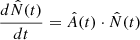 (A.1)
(A.1)
where  is the vector of level populations over all ions (ΣiNi(t) = 1) and
  is the rate matrix. The initial condition
  corresponds to the steady state equilibrium at ne = 10−3 cm−3 and Te = 7 keV. The time steps were chosen on a logarithmic scale via: t0 = 0, t1 = 104 s, and ti + 1 = ti ⋅ 1.2 for i = 1..169 (t169 = 2.408 ⋅ 1017 s). At each time step between i = 0 and i = 21, the electron temperature increased by 1 keV until reaching 28 keV at t21 = 3.834 ⋅ 105 s, after which it was kept constant. The calculated ion populations and line intensities for He-like and H-like lines are shown in Figs. 2 (open squares) and 4, respectively. The relative population influxes for Z and W lines are presented in Fig. A.1 while the absolute influxes are given in Fig. A.2. For the frozen ionization distribution at relatively small τ, an instantaneous increase of the electron temperature results in a mildly enhanced excitation influx for the W line. Although Z also experiences an increased influx due to the inner-shell ionization from the ground state of Fe23+, the relatively small population of the latter cannot provide an influx increase comparable to that for W. Hence, the Z/W ratio decreases as compared to the low-temperature condition.
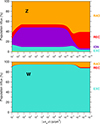 |
Fig. A.1. Relative population influxes for Z and W lines (T0 = 7 keV, T1 = 28 keV, Te = Tp case). RAD: radiative cascades, REC: direct radiative recombination from the H-like ground state, ION: inner shell ionization from the Li-like ion, EXC: electron-impact excitation. |
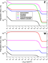 |
Fig. A.2. Absolute population influxes for Z and W lines (T0 = 7 keV, T1 = 28 keV, Te = Tp case). |
For the second set of calculations, the initial temperature (T0) was set in the 1..50 keV range. Then, the temperature (T1) was changing from 1 keV to 50 keV with a time step of 104 s. This time step is too short to modify abundances of the ions involved while long enough to ensure quasi-steady-state equilibration between the excited states within an ion, which is established on the times compared to the longest lifetimes (cf. τ ≃ 5 ⋅ 10−9 s cm−3 for the Z line). Then, the corresponding Z/W ratio was determined for the combination of (T0, T1) as shown in Fig. 3. After the fast rise of electron temperature, the contribution of the inner shell ionization from the ground state 1s22s of the Li-like ion to the Z influx increases by about a factor of four and remains high until the progressive ionization begins to deplete Li-like ions at about τ ∼ 1010 s cm−3 (Figs. A.1 and A.2).
Appendix B: Reference list for the relevant lines
In Table B.1, we list key parameters of the lines considered in this study for reference.
Key parameters of the most relevant lines.
Appendix C: Role of Helium in temperature equilibration
In this section, we verify the impact of helium on the ion temperature evolution, considering energy exchange between electrons, protons, helium ions, and ions of Fe XXV. The same assumption of a pure adiabatic heating of electrons at the shock is made. The subsequent evolution is mediated by Coulomb collisions. Fig. C.1 compares the evolution with helium (dashed lines) and without helium (solid lines). In the former case, the initial downstream temperature of ions is lower because of the increased mean atomic weight of plasma and, therefore, slower shock velocity (for the same upstream temperature and the shock Mach number), reducing the nonadiabatic heating of ions. Conversely, at later times (τ > 1012 cm−3 s), the presence of He ions keeps the Fe XXV ions slightly hotter, because He ions have the longest equilibration time scale.
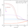 |
Fig. C.1. Impact of helium on the temperature equilibration. The solid lines correspond to the case with no helium, while the dashed lines show the temperature evolution when the He abundance is set to 0.084 of hydrogen (Lodders et al. 2009). The main effect of helium is (i) the increase of the mean atomic weight of plasma and, as a consequence, lower downstream temperature of ions (visible for τ < 1012 cm−3 s) and (ii) keeping Fe ions slightly hotter at τ > 1012 cm−3 s, since the helium ions have the longest equilibration time. |
All Tables
All Figures
|
Fig. 1. Coulomb-collision-mediated temperature equilibration between electrons, protons, and He-like iron ions (Fe XXV) in the limit of adiabatic heating of electrons at the shock. The Fe XXV ions temperature, TZ, approaches Tp at τ ∼ 1012 cm−3 s and then evolves together with Tp. The NEI timescale (see Fig. 2 below) is approximately the same as the TZ ≫ Tp timescale. Ions remain hotter than electrons up to τ ∼ 2 − 3 × 1013 cm−3 s. Therefore, the Fe XXV ions are hotter than Te up to this value of τ, and the thermal broadening of the Fe XXV lines is larger than that predicted from the electron temperature Te derived from the continuum shape. The helium abundance is set to zero for this plot (see Fig. C.1 for the impact of helium). |
| In the text | |
|
Fig. 2. Ionization balance and temperature evolution in the shocked medium. Bottom: Evolution of Te. The solid blue line corresponds to the Te = Ti = const case, while the dashed red line shows the “Coulomb” temperature equilibration, with Te initially set by adiabatic compression in the ℳ = 3.2 shock. In this case, Te rises slowly and does not reach Tp even at τ = 1012 cm−3 s. Top: Evolution of ionization balance. Solid lines show the Te = Ti case, based on CHIANTI rates, and open squares show the NOMAD results. Dashed lines show the ion fraction evolution when the electron temperature itself evolves with time, as shown in the bottom panel. |
| In the text | |
|
Fig. 3. Simulated Z/W line intensity ratio (colors; NOMAD simulation) for an instantaneous change in electron temperature from T0 to T1 in the limit of small τ. Locations a and c correspond to the flux ratios for the initial and final states with T = 7 keV and T = 28 keV, respectively. The dashed diagonal line shows the locus of other equilibrium states with T1 = T0. Location b corresponds to the intermediate case with T0 = 7 keV, T1 = 28 keV, and τ = 1010 cm−3 s. A similar ratio is expected over a wide range of τ ≲ 3 × 1010 cm−3 s. This transient state with an anomalously low Z/W ratio may serve as a signature of freshly shocked hot NEI plasma. |
| In the text | |
|
Fig. 4. Time-dependent (a) line intensities and (b) line intensity ratios for He- and H-like Fe from the NOMAD simulation (T0 = 7 keV, T1 = 28 keV, Te = Tp case). The 0.25 scaling factor applied to the W/Lyα ratio places all data on the same scale. Solid circles show the corresponding values at τ = 0, i.e., T0 = 7 keV. |
| In the text | |
|
Fig. 5. Left: Evolution of Z/W (solid lines) and Ly/W (dashed lines) ratios following an instantaneous (black) and Coulomb-collisions-mediated (red) increase in electron temperature from 7 to 28 keV (corresponding to ℳ = 3.2 shock). The dashed blue line shows the ratio for a kT = 7 keV CIE plasma. Right: Same as in the left panel but for an initial temperature of 6.5 keV and a final temperature of 12 keV (corresponding to a ℳ = 1.8 shock). While the Z/W flux ratio differs between the Te = Tp and Te < Tp cases, it remains lower than the CIE-predicted values. The evolution of the Ly/W ratio is driven primarily by time-dependent changes in the ionization balance. |
| In the text | |
|
Fig. 6. Triplet spectrum for different assumptions about the ion temperature and different ionization parameter τ. Left: Case with τ = 1011 cm−3 s. The red, blue, and brown curves show TZ = Te, TZ = Tp, and |
| In the text | |
|
Fig. 7. Emission measure EMτ of shocked gas with the ionization parameter τ below a given threshold, relative to the emission measure EMcl of unshocked gas at the same distance from the cluster center (see Eq. 7). The solid and dashed purple lines show the ratio EMτ/EMcl for τ = 1011 and 1012 cm−3 s, respectively. For the shock velocity, we use the velocity vr of a point mass on a parabolic orbit. The blue and red lines show the overdensity of baryons as a function of radius and the product of overdensity and radius, respectively. The reciprocal of the latter quantity is the key quantity that determines the ratio EMτ/EMcl. The plots show that regions with τ ∼ 1011 cm−3 s can contribute ∼10% to the line-of-sight emission measure, while for τ ∼ 1012 cm−3 s the contributions from shocked and unshocked regions can be comparable. This conclusion holds for essentially any projected distance from the cluster center, although projection effects may also play a role. |
| In the text | |
|
Fig. A.1. Relative population influxes for Z and W lines (T0 = 7 keV, T1 = 28 keV, Te = Tp case). RAD: radiative cascades, REC: direct radiative recombination from the H-like ground state, ION: inner shell ionization from the Li-like ion, EXC: electron-impact excitation. |
| In the text | |
|
Fig. A.2. Absolute population influxes for Z and W lines (T0 = 7 keV, T1 = 28 keV, Te = Tp case). |
| In the text | |
|
Fig. C.1. Impact of helium on the temperature equilibration. The solid lines correspond to the case with no helium, while the dashed lines show the temperature evolution when the He abundance is set to 0.084 of hydrogen (Lodders et al. 2009). The main effect of helium is (i) the increase of the mean atomic weight of plasma and, as a consequence, lower downstream temperature of ions (visible for τ < 1012 cm−3 s) and (ii) keeping Fe ions slightly hotter at τ > 1012 cm−3 s, since the helium ions have the longest equilibration time. |
| In the text | |
Current usage metrics show cumulative count of Article Views (full-text article views including HTML views, PDF and ePub downloads, according to the available data) and Abstracts Views on Vision4Press platform.
Data correspond to usage on the plateform after 2015. The current usage metrics is available 48-96 hours after online publication and is updated daily on week days.
Initial download of the metrics may take a while.