


| Issue |
A&A
Volume 711, July 2026
|
|
|---|---|---|
| Article Number | A284 | |
| Number of page(s) | 13 | |
| Section | Stellar structure and evolution | |
| DOI | https://doi.org/10.1051/0004-6361/202660357 | |
| Published online | 23 July 2026 | |
The applicability of the JAGB method for measuring the distance of galaxies subject to different metal-enrichment rates
1
Dipartimento di Matematica e Fisica, Università degli Studi Roma Tre, Via della Vasca Navale 84, 00100 Roma, Italy
2
INAF, Observatory of Rome, Via Frascati 33, 00077 Monte Porzio Catone (RM), Italy
3
Dipartimento di Fisica, Sapienza, Università di Roma, Piazzale Aldo Moro 5, 00185 Roma, Italy
4
ASI-Space Science Data Center, Via del Politecnico, I-00133 Rome, Italy
5
Istituto Nazionale di Astrofisica– Osservatorio Astronomico di Padova, Vicolo dell’Osservatorio 5, I-35122 Padova, Italy
★ Corresponding author: This email address is being protected from spambots. You need JavaScript enabled to view it.
Received:
10
April
2026
Accepted:
9
May
2026
Abstract
Context. The JAGB method has been proposed over the last years as a possible distance indicator for galaxies in the Local Group and beyond. The nature of the stars populating the J region, as well as the conditions of the star formation history and the structural properties of the galaxies for the direct application of this method, still needs to be investigated.
Aims. We aim to assess the robustness of the JAGB method in measuring the distance of galaxies, presenting a detailed theoretical analysis of the stars populating the J region of the (J − KS, J) diagram. The primary goal of the present analysis is to identify the properties of the corresponding J luminosity function (JLF) that are insensitive to the metal-enrichment history of the interstellar medium and may therefore provide robust distance indicators.
Methods. We used a population synthesis approach, based on extant stellar models of asymptotic giant branch evolution coupled self-consistently with the description of the dust formation process in the wind. This was done to build synthetic distributions of stars on the (J−KS,J) diagram and to calculate the corresponding JLF of the stars in the J region. The simulations were repeated for different hypotheses regarding the time variation of the metallicity of the interstellar medium in order to study the sensitivity of the JLF to the timescale of the metal-enrichment process.
Results. The statistics of the J region is mostly determined by the stars formed between ∼6 Gyr and ∼1 Gyr ago, because stars formed outside this time interval barely enter the JAGB box. The shape of the JLF changes significantly with the metal-enrichment, in particular through variations in the peak J magnitude, which changes over a range exceeding 0.3 mag. Conversely, the mean J magnitude, MJav, proves much less dependent on the previous history of the galaxy and thus a much more robust distance indicator: we find MJav = −6.2 ± 0.05 mag for all the cases investigated. The uncertainties connected to the still largely unknown process of mass loss suffered by low-mass stars during the evolution along the red giant branch are also commented on.
Key words: stars: AGB and post-AGB / stars: carbon / stars: evolution / stars: mass-loss / distance scale
© The Authors 2026
 Open Access article, published by EDP Sciences, under the terms of the Creative Commons Attribution License (https://creativecommons.org/licenses/by/4.0), which permits unrestricted use, distribution, and reproduction in any medium, provided the original work is properly cited.
This article is published in open access under the Subscribe to Open model. This email address is being protected from spambots. You need JavaScript enabled to view it. to support open access publication.
1. Introduction
In the last decades we have witnessed a growing interest in the stars evolving through the asymptotic giant branch (AGB), owing to their efficiency as pollutants of the interstellar medium and the important role they play in the chemical enrichment of galaxies through their cosmic evolution history (Kobayashi et al. 2020; Romano 2022), including the formation of multiple populations in globular clusters (Ventura et al. 2001). Further interest in this class of objects arose when they were recognized as being among the most efficient dust manufacturers, also providing a significant contribution to the dust production in the high-redshift Universe (Valiante et al. 2009, 2011; Mancini et al. 2015; Ginolfi et al. 2018; Aoyama et al. 2018; Graziani et al. 2015; Schneider & Maiolino 2024).
Stellar modelers recently included the description of the dust formation process in the wind of cool stars, thus making it possible to determine the dust production rate (DPR) of stars, as they evolve along the AGB (Ventura et al. 2012, 2014; Nanni et al. 2013, 2014). These efforts have been dictated not only by the need to infer the mineralogy and the amount of dust produced by AGB stars, but also to understand the evolution of their spectral energy distribution (SED), given the reprocessing of the radiation released by the photosphere by the dust particles present in the circumstellar envelope. The coupling of dust formation with stellar evolution modeling is essential for the computation of the evolutionary tracks of stars of different masses and metallicities across observational color-magnitude diagrams (CMDs) built with near-infrared (NIR) and mid-infrared (MIR) filters. This approach was used to characterize the evolved stellar populations of the Magellanic Clouds (MCs) (Dell’Agli et al. 2014b; Dell’Agli et al. 2015a,b; Nanni et al. 2016, 2018, 2019), of a few Local Group (LG) galaxies (Dell’Agli et al. 2016; Dell’Agli et al. 2018; Dell’Agli et al. 2019), and Andromeda (Gavetti et al. 2025).
An accurate description of the evolution of AGB stars and of dust formation in their winds is more essential than ever, now that we are in the James Webb Space Telescope (JWST) era. Indeed, the JWST enables the detection of resolved stellar populations in galaxies well beyond the LG and provides an exceptional tool for studying AGB stars (Correnti et al. 2025; Bortolini et al. 2025). For a significant fraction of these systems, AGB stars represent important tracers for reconstructing their star formation histories (SFHs), owing to their age sensitivity in the NIR (Lee et al. 2024; Bortolini et al. 2024). In this regard, recent studies have outlined the potential offered by the number counts of evolved stars in reconstructing the SFH of galaxies, a method that has only been applied to the Milky Way satellites so far, based on Hubble Space Telescope (HST) data (Harmsen et al. 2023).
The use of AGB stars, or at least some of them, as distance indicators of galaxies, was recently added to the themes discussed above and further underlines the need for an exhaustive understanding of the evolutionary properties of these objects. This is the so-called J-asymptotic giant branch (JAGB) method, first proposed by Nikolaev & Weinberg (2000), who suggested using the AGB stars located in a rectangular box of the (J − Ks, Ks) diagram of the Large Magellanic Cloud (LMC), later called the “J region”, as standard candles. An accurate calibration of the JAGB method would lead to the measurement of the distances of galaxies that are found to be further away than those already determined using other methods. Indeed, JAGB stars are significantly brighter on average than the tip of the red giant branch (TRGB), allowing distance determinations well beyond the TRGB limit. Compared to Cepheids, the JAGB method requires only a single epoch of observations, and it can be applied to galaxies hosting stellar populations with ages between ∼200 Myr and 1 Gyr, whereas Cepheids are confined to the disks of spiral and irregular systems.
While the initial investigations were based on the MCs, following works investigated the J luminosity functions (JLFs) of other galaxies, and confirmed that the applicability of the JAGB method can be considered as general. Important contributions in this field came from Madore & Freedman (2020) and Freedman & Madore (2020), who studied the JLFs of 16 galaxies, finding that all the JLFs can be approximated by a nearly mono-modal, slightly asymmetric Gaussian function, which peaked at MJ = −6.2 mag, with a small scatter on the order of 0.02 mag. A more recent and exhaustive investigation was presented by Freedman et al. (2025), which focused on the JLFs of 70 galaxies observed in the I band, and found little evidence supporting multimodal fits. Further applications of this technique to other galaxies were presented by Lee et al. (2024) and Li et al. (2025).
Magnus et al. (2024) recently refined the calibration of the JAGB method using Gaia data on the MCs, selecting a clean carbon star sample within 1.5 < J−K < 2.0 mag and a 1.2 mag wide J window: they found a mean MJ of ∼ − 6.25 mag for the LMC and ∼ − 6.18 mag for the Small Magellanic Cloud (SMC). Gavetti et al. (2026) applied stellar evolution modeling of AGB stars, coupled with the description of dust formation, to interpret the results obtained by Magnus et al. (2024), and they successfully reproduced the JLFs derived by Magnus et al. (2024) for the LMC and the SMC. The analysis by Gavetti et al. (2026) outlined that the population of the J region is composed of stars evolving through a well-defined evolutionary phase during the AGB, that extends from the early phases following the C star stage until the amount of carbon dust in the circumstellar envelope becomes large enough to shift the SED entirely to the MIR region, so that they move to the J−K > 2.0 mag region of the CMD. An important side result obtained by Gavetti et al. (2026) is that the possibility of stars evolving into the J region and the amount of time spent there are extremely sensitive to the progenitor’s mass and to the metallicity. Because stars of different masses and metallicities nowadays evolving along the AGB formed in different epochs, the results obtained by Gavetti et al. (2026) show that the numerical consistency and the distribution of the stars in the J region are tightly connected to the previous history of galaxies, in terms of the metal-enrichment of the interstellar medium and of the SFH.
A more general approach is required to test the applicability of the JAGB method to galaxies other than the LMC and SMC, where no a priori choice of the SFH is made: this is the only way to explore the conditions under which the JAGB method can be universally applied to measure the distances of galaxies. The present research project is aimed at providing a critical evaluation of the applicability of the JAGB method in relation to the type of galaxies investigated. One of the objectives of this study is to test whether some properties of the JLFs of the stars, for example the mean and the peak J magnitudes, are independent of the previous history of metal-enrichment of the galaxies.
In this work, we used the same approach adopted in Gavetti et al. (2026) to produce synthetic distributions of stars in order to study the population of the J region in detail. We focused on the role played by the metal-enrichment, varying the rate at which the metallicity of the interstellar medium increases over time. While the evolution of different galaxy types is generally characterized by different SFHs, in the present analysis we assume a constant star formation rate (SFR) during the various epochs for the sake of simplicity; a more general analysis, where changes in the SFR are taken into account for different classes of galaxies, will be the subject of a forthcoming paper. Part of the study is devoted to the relevance of the assumptions regarding the mass loss experienced by low-mass stars during the red giant branch (RGB) evolution: this point is often neglected in the literature, despite it being shown to be crucial for the interpretation of the evolved stars’ distribution in the galaxies on the observational diagrams (Gavetti et al. 2025) and to heavily affect the number counts and the relative fraction of AGB over RGB stars in the Milky Way satellites (Ventura et al. 2026).
This paper is structured as follows: the physical and numerical ingredients used for the simulations are described in Sect. 2; in Sect. 3 we discuss the general properties of the AGB evolution of stars of different masses and metallicities, and the time spent in the J region; the sensitivity of the shape of the JLF to the timescale of the metal-enrichment of the galaxies is addressed in Sect. 4; Sect. 5 is devoted to the analysis of the applicability of the J method to infer the distance of galaxies; finally, the conclusions are given in Sect. 6.
2. Physical and numerical input
The present work is based on results obtained through a population synthesis approach. Artificial distributions of stars in the CMD of a given galaxy were simulated according to specific assumptions about their SFHs that characterize the time from the galaxy’s formation to the present day. As stated in the previous section, the main goal of the present investigation is the study of how the metal-enrichment affects the population of the J region of the CMD. Therefore, as a first approach, we assumed a constant SFR, while the metallicity of the gas increases over a timescale that was varied among the different simulations.
It should be noted that proper assumptions regarding the SFH should be based first on the galaxy type under investigation (Conroy 2013; Madau & Dickinson 2014); second on their physical properties, i.e., mainly their stellar mass (Pacifici et al. 2016); and finally on their dynamical and environmental evolution. While a constant SFH with SFR variations of a factor of two to three over the past few gigayears was quite a common assumption in early studies of some irregular and dwarf galaxies (Marconi et al. 1995; Grebel 2020), recent observations have also shown a variety of possible SFHs for small irregular objects, which are generally fragile to feedback processes (see Tolstoy et al. 2009 and references therein). For dwarf galaxies, both within the LG and beyond, a fairly moderate star formation activity can generally be assumed when averaging over sparse episodes. In the case of classical spiral galaxies of the LG, this assumption should generally be limited to an interval of their global evolution. This also depends on assumptions about quenching efficiency, and a more general log-normal SFH appears more appropriate when compared with the predictions from numerical simulations (Diemer et al. 2017). The above assumptions are certainly less appropriate for elliptical galaxies as their old stellar populations are often interpreted in terms of strong initial bursts followed by a long evolution without star formation episodes (Rogers & Ferreras 2010); however, recent studies suggest that their stellar populations may be more complex (Jegatheesan 2025). A common assumption is then not applicable to heterogeneous samples. Semi-analytical models, for example, tend to reduce the parameter space when modeling SFHs of heterogeneous samples by assigning simple functional forms to each type (Calura et al. 2004). With the above caveats, we started our investigation with an oversimplified assumption of a constant SFH while deferring a more realistic galaxy-type-dependent treatment to future work.
To produce the synthetic populations, we followed the same methodology introduced by Dell’Agli et al. (2014a, 2015a) and applied by Gavetti et al. (2025, 2026), which can be summarized into four steps, listed and briefly discussed below.
-
The evolutionary sequences, calculated by means of the ATON code for stellar evolution (Mazzitelli 1979; Ventura et al. 1998), are taken from the Rome library and were published and discussed in Ventura et al. (2014), Ventura et al. (2018), Marini et al. (2021), Kamath et al. (2023). For the present investigation we used stellar models of metallicities Z = 1, 2, 4, 8 × 10⁻³, 1.4 × 10⁻², which correspond to the −1.5 ≤ [Fe/H] ≤ 0 range. For stars of mass 2 M⊙ < M < 8 M⊙ the evolutionary sequences were started from the pre-MS phase and evolved until the end of the AGB, when almost the entire envelope was lost. For stars with M ≤ 2 M⊙ the evolutionary sequences were first evolved from the pre-MS until the helium flash, then were resumed from the core helium-burning phase, with the same core mass reached at the occurrence of the helium flash. For the latter sequences, started from the core helium-burning, an assumption must be made regarding the amount of mass lost during their ascent along the RGB, which we will denote as δmRGB. The results presented here were obtained with δmRGB = 0.2 M⊙. This choice is motivated by several investigations on the stellar populations of globular clusters, which demonstrated that RGB mass losses of the order of 0.2 M⊙ are required to reproduce the various observational features, particularly the morphology of the horizontal branch (Tailo et al. 2021). The effects of different choices of δmRGB are discussed in Sect. 4.4. The results from stellar evolution modeling allow us to follow the time variation of the main physical quantities of the star, namely mass, luminosity, effective temperature, mass-loss rate, and of the surface chemical composition, during their evolution.
-
For the evolutionary sequences discussed in the previous point, dust formation in the wind is modeled, following the same approach used in previous works on this topic (Ventura et al. 2012, 2014, 2018; Gavetti et al. 2025, 2026). We apply the chemo-dynamical description of the wind proposed by Ferrarotti & Gail (2002, 2006) to some evolutionary stages chosen along the AGB (typically, we select 20 points during the early-AGB and 10 points between two consecutive thermal pulses (TPs) of the TP–AGB evolution, approximately equally spaced in time). The values of the luminosity, effective temperature, current mass, and mass-loss rate corresponding to the selected evolutionary stages, found as described in point 1), are used as ingredients to model the formation and growth of the dust grains, adopting the set of equations described in detail in Ventura et al. (2012). The types of dust species considered depend on the surface chemical composition: for oxygen-rich environments we consider the formation of silicates, alumina dust and solid iron, while for carbon stars we model the growth of amorphous carbon, silicon carbide and solid iron. This step leads to the determination of the overall DPR, of the asymptotic size reached by each dust species, of the percentage contribution of each dust species to the global dust formed in the circumstellar envelope, and of the optical depth (similarly to previous investigations, here we consider the value at a wavelength of 10 μm, τ10), for each of the evolutionary stages considered.
-
The dust mineralogy and the values of τ10 found in point 2) are used to find the synthetic SED for each of the evolutionary stages considered. This step is performed using the DUSTY code (Nenkova et al. 1999). Convolving the synthetic SED with the transmission curves of the observational filters enables the computation of the evolutionary tracks for the model stars of different mass and metallicity in the various CMDs of interest. In the present investigation, as discussed in the previous section, we focus on the (J−Ks,J) CMD.
-
The final step consists of constructing a synthetic distribution of stars in the CMD, using a population synthesis approach, as described in Gavetti et al. (2025). Briefly, we consider the time evolution since 14 Gyr ago to the present, assuming, as discussed above, that the SFR has been constant across the various epochs, and that the initial mass function (IMF) is described by a Kroupa (2001) law. The timescale of metal-enrichment, τZ, is used as a free parameter. The distribution of stars on the CMD is found by considering the time evolution of stars of different masses and metallicities, and then by interpolation among the different tracks, calculated as described in point 3) above.
For the construction of the synthetic populations discussed in this section, we adopted a SFH characterized by a SFR of 0.3 M⊙/yr extended over the entire life of the galaxy (14 Gyr). This choice results in a total stellar mass of approximately 4.2 × 10⁹ M⊙, which ensures that the J region is populated by a statistically robust sample of artificial stars. We emphasize that the resulting morphology of the JLFs, as well as the determination of key parameters such as the mean and peak J magnitudes, are numerically independent of the specific choice of the SFR value. From an astrophysical standpoint, the relative shape of the JLF is fundamentally determined by the product of the IMF and the evolutionary crossing times (τJAGB) of stars with different masses and metallicities. Since the SFR acts primarily as a global normalization factor, changing its value scales the total number of stars but does not alter their relative distribution across magnitude bins, provided the total number of stars is sufficiently large to minimize stochastic Poissonian fluctuations.
3. The role of mass and metallicity in the carbon enrichment and infrared colors of AGB stars
Ventura et al. (2022) divided AGB stars into three groups, distinguished based on the modification of the surface chemical composition. Group I consists of low-mass stars, which, after only a few third dredge-up (TDU) events, lose the external envelope when the surface C/O is still below unity. This behavior is common to the stars that start the core helium-burning phase with a mass below a threshold value of Mcarb, i.e., on the order of 1 M⊙, which increases with the metallicity (Kamath et al. 2023); this is because metal-poor stars become C stars more easily, owing to the low initial oxygen content. Group II includes stars with masses between Mcarb and an upper threshold of MHBB ∼ 3−4 M⊙, which become carbon stars during the AGB phase. In these stars the surface carbon gradually increases during the entire AGB lifetime, owing to repeated TDU events, until the envelope is lost. Group III is composed of massive AGB stars of initial masses above MHBB. These stars experience hot bottom burning (HBB) (Sackmann & Boothroyd 1992; Blöcker & Schönberner 1991), a process that destroys carbon nuclei via proton-capture nucleosynthesis at the base of the convective envelope. Consequently, these stars do not become C stars. MHBB decreases with metallicity, as HBB is activated more easily in metal-poor stars (Dell’Agli et al. 2018).
The stars belonging to the three groups populate different regions of the CMD: this is due partly to the obvious differences in the luminosities, which increase with the progenitor’s mass, and partly to the fact that the path followed by the evolutionary tracks is highly sensitive to whether and when the stars reach the C star stage. Indeed, the achievement of the C/O > 1 condition is accompanied by a significant increase in the surface molecular opacities (Marigo 2002), which triggers the expansion and cooling of the surface regions and, consequently, the increase in the mass-loss rate and in the density of the wind. These conditions become extremely favorable to the formation of carbon dust, which effectively starts when the carbon excess with respect to oxygen exceeds ∼10%, so there is a sufficiently large number of carbon molecules available to condense into carbon grains1. The formation of carbon dust causes the SED to shift toward the NIR and MIR spectral regions, so the stars evolve toward the red side of the CMD.
Since most, if not all, of the stars in the J region are carbon stars, in the present analysis we focused our attention on the stars belonging to group II. Group III stars are indeed of little interest for the comprehension of the stellar population of the J region, because they are too bright to populate the box suggested by Magnus et al. (2024) to define the J region, and their statistical weight would be negligible even if a different box were chosen, given their short evolutionary timescales. Even the stars in group I, which never become C stars, rarely enter the J region due to their low dust production, with the sole exception of the solar metallicity case, which is discussed in the following sections.
3.1. The start and the timescale of the surface carbon enrichment
As the formation of carbonaceous dust begins when there is a sufficiently large excess of carbon with respect to oxygen in the surface regions of the star, the key parameter determining whether a star enters the J region during its evolution is the surface C/O ratio. The variation of this quantity during the AGB phase for stars of different masses and chemical compositions is shown in Fig. 1. Stars of different metallicities evolving on timescales of 1, 3, and 5 Gyr are shown in the left, middle, and right panels, respectively. This comparison, aimed at identifying when stars of different ages and metallicities become C stars, is extremely important for understanding the contribution of stars formed during the various epochs to the population of the J region.
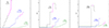 |
Fig. 1. Time variation of the surface C/O ratio of model stars of metallicity Z = 10−3 (black lines), Z = 4 × 10⁻³ (blue), and Z = 0.014 (green) that formed ∼1 Gyr ago (left panel), ∼3 Gyr ago (middle), and ∼5 Gyr ago (right). The magenta portion of the lines indicates the phases during which the model stars cross the J region. The horizontal gray lines indicate the time when the stars become C stars. Times are counted from the beginning of the TP–AGB phase. The masses reported in the middle and right panels refer to the start of the core helium-burning phase. |
For stars formed 1 Gyr ago, we considered model stars with masses of 2 M⊙, 2.25 M⊙ and 2.5 M⊙ for the Z = 10−3, Z = 4 × 10⁻³ and Z = 0.014 cases, respectively. These stars accumulate the largest amounts of surface carbon, whose mass fractions eventually exceed 1%. Dell’Agli et al. (2015a) associated the reddest sources populating the color–color ([3.6]−[4.5],[5.8]−[8.0]) diagram of the LMC with the late evolutionary phases of these objects, and concluded that they provide the most significant contribution to the overall DPR of the galaxy. Their peculiarity arises from the fact that they reach the C star stage after only a small fraction of the envelope mass is lost. Consequently, they experience several TPs after becoming C stars, allowing the surface carbon abundance–and therefore the DPR–to increase considerably. The fraction of the AGB lifetime spent as a C star decreases from ∼80% for the Z = 10−3 model star to ∼15% in the solar case. This is because higher-metallicity stars form with a larger initial oxygen abundance, which hinders the achievement of the C star stage.
Regarding the stars formed 3 Gyr ago, the model stars reported in the middle panel of Fig. 1 are characterized by masses at the start of the core helium-burning phase of 1.1 M⊙, 1.25 M⊙, and 1.5 M⊙, for the Z = 10−3, Z = 4 × 10⁻³, and Z = 0.014 cases, respectively. The most relevant difference with respect to the higher-mass counterparts, discussed above, is that these stars only become C stars during the final part of the AGB phase; thus, they only experience a few TDU events after the surface C/O ratio exceeds unity in the surface regions. Consequently, the fraction of the AGB lifetime spent as a C star is significantly shorter than for their 1 Gyr counterparts, and the final C/O ratios are smaller. In the specific case of the solar-metallicity model star, the C star phase is limited to the last two inter-pulse phases, and the fraction of time spent as a C star is below 10%.
Finally, in the case of the low-mass stars formed 5 Gyr ago, the effect of metallicity becomes even more important than in the cases discussed above. Indeed, only the metal-poor model star (with an initial mass of 0.9 M⊙ at the start of the core helium-burning phase) spends a non-negligible fraction (∼25%) of the AGB lifetime as a C star, while the 0.95 M⊙ model star of Z = 4 × 10⁻³ only becomes a C star when the last TP takes place. The solar-metallicity model star of mass 1.1 M⊙ fails to reach the C star stage.
3.2. The evolutionary tracks on the (J−Ks,J) diagram
As discussed earlier in the present section, the change in the surface chemical composition, particularly in the C/O ratio, affects the morphology of the evolutionary tracks on the CMD. Some selected tracks of stars of different masses and metallicities are shown in Fig. 2. Each point along the tracks corresponds to a specific stage during the inter-pulse phase, when the luminosity attains the maximum value: thus, the spacing between the points indicates how fast the tracks move across the CMD.
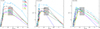 |
Fig. 2. Evolutionary tracks of stars of different masses and metallicities in the color–magnitude (J−KS,J) diagram. For M≤ 2 M⊙ the masses were taken at the beginning of the core helium-burning phase. The points along each track refer to the phases of maximum luminosity experienced during an inter-pulse phase. Open symbols refer to the phases during which the star is O-rich, whereas full points indicate C-rich phases. The gray shaded box indicates the J region defined by Magnus et al. (2024). |
In general, the evolutionary tracks move vertically during the first part of the AGB evolution, during which they are practically dust-free, and the J flux increases as a consequence of the gradual rise in the luminosity. When carbon dust formation begins, the tracks move to the red due to the gradual shift of the SED to the NIR. The J flux increases until (J−Ks) ∼ 1.7 mag and then decreases, because the peak of the SED moves to wavelengths of λ > 1 μm as carbon accumulates in the surface layers of the star and the DPR increases. The only exceptions to this common behavior are the 3 M⊙ model stars of metallicity Z = 10−3, 4 × 10⁻³ and the M ≤ 1 M⊙ model stars of solar chemical composition; in these cases the redward excursion of the evolutionary tracks is associated with the formation of silicates. The theoretical necessity of including dust formation to explain the NIR colors of the JAGB population is strongly corroborated by observational evidence. If we consider, for example, the spectroscopically confirmed carbon stars (Wood et al. 2013) populating the J region, they show dust features (e.g., silicon carbide emission) in their spectra.
The metallicity effects can be deduced by comparing the morphology of the evolutionary tracks of low-mass stars of different Z. For the reasons given before, metal-poor stars become C stars after experiencing only a few TPs; during this time, the core mass, and hence the luminosity, are lower than in the higher-metallicity counterparts. This is reflected in the J flux at which the transition to the red side of the CMD takes place; this flux becomes progressively fainter as the metallicity decreases.
3.3. The crossing time of the J region
Characterizing the stellar population of the J region requires knowledge of the amount of time that the stars spend in that part of the CMD. As discussed earlier in this section, the stars evolve within this region of the CMD during an intermediate evolutionary phase, which starts soon after the C star stage is achieved and lasts until the DPR attains values so large that the (J−Ks) colors increase, the J flux decreases, and the stars no longer populate the JAGB box.
Figure 3 shows the times τJAGB spent in the J region of the CMD by model stars of different masses and metallicities as a function of the initial mass (left panel) and of the formation epoch (right). As discussed in Gavetti et al. (2026), the stars spending the longest time within the JAGB box, that is, slightly below 1 Myr, are the progeny of 2−2.5 M⊙ stars, which formed ∼1 Gyr ago. This is consistent with the discussion of Sect. 3.1 and is related to the fact that these objects reach the C star stage when only a small fraction of the envelope is lost; thus, the increase in the surface carbon is gradual and the transition to the very red side of the CMD is delayed. This can also be seen in Fig. 2, where we note that the evolutionary tracks of 2−2.5 M⊙ stars remain within the JAGB box for several inter-pulse phases.
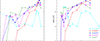 |
Fig. 3. Times spent within the J region by model stars of different masses and metallicities as a function of the progenitor’s mass (left panel) and of the formation epoch (right). The masses for M ≤ 2 M⊙ stars refer to the start of the core helium-burning phase. For masses below 1.5 M⊙ we considered an average mass loss during the RGB evolution of 0.2 M⊙; thus, the formation epochs reported on the abscissa of the right panel refer to those of the model stars of mass 0.2 M⊙ higher than those reported on the abscissa of the left panel. Each sequence is limited to the masses whose evolutionary tracks enter the J region. |
As far as subsolar metallicities are concerned, the τJAGB versus mass trend is positive, given the small fraction of time during which low-mass stars evolve as C stars; this can be deduced by comparing the results shown in the middle and right panels of Fig. 1 with those reported in the left panel of the same figure. We note in Fig. 2 that the evolutionary tracks of low-mass stars stay within the JAGB box for at most two inter-pulse phases, before moving toward the red, low-luminosity side of the plane. Solar-metallicity model stars are an exception to this general behavior, because after becoming C stars they cross the J region very fast, owing to the rapid expansion and cooling of the outermost regions. Unlike the lower-metallicity cases, the stars spending the longest time within the J region (∼ 2 × 10⁵ yr) are the progeny of stars with masses of 1−1.2 M⊙: these stars evolve into the J region during the final AGB phases, when they are oxygen-rich, and the redward excursion of the evolutionary tracks is due to the formation of silicates in the circumstellar envelope; this is in turn favored by the cool surface temperatures and the significant amount of gaseous silicon.
The slope of the τJAGB versus mass (or formation epoch) relation reported in Fig. 3 is significantly affected by the metallicity: this trend, discussed in Gavetti et al. (2026), is due to the fact that metal-rich, low-mass stars reach the C star stage only after a significant fraction of the envelope is lost and thus only evolve as C stars during the very final AGB phases. As metallicity decreases, lower-mass stars become C stars more easily and at earlier stages of the AGB evolution. Consequently, the time spent within the J region by low-mass stars increases significantly in metal-poor environments. This can be deduced by comparing the fraction of time spent in the C star phase by the model stars of different metallicity in the middle and right panels of Fig. 1.
The results presented so far indicate that the vast majority, if not all, of the stars populating the J region formed between 1 and 6 Gyr ago. This is the time interval of interest for a critical evaluation of the various factors entering the characterization of the stars in the JAGB box and affecting their luminosity distribution. In environments characterized by subsolar metallicities, the star formation that occurred around 1 Gyr ago is crucial to determining the numerical consistency of the sample of stars within the J region, because that is the formation epoch of the stars that spend the longest time in that region, namely the progeny of 2−2.5 M⊙ stars. By contrast, we expect the JAGB population of galaxies that reached solar metallicity more than 1–2 Gyr ago to differ significantly from that of other systems, owing to the peculiar behavior of solar-metallicity stars.
4. The J luminosity function of the stars in the J region
The arguments presented in the previous section provide the key elements for understanding how stars evolve into the J region, and thus how the expected JLF changes according to the SFH and the chemical enrichment history of galaxies. As discussed in Sects. 1 and 2, in the present analysis we applied the population synthesis approach described in Sect. 2 to galaxies where the SFR was constant and the metal-enrichment of the interstellar medium proceeded on different timescales. We started from the basic case, where no metal-enrichment occurred, and extended the analysis to the case in which the metal-enrichment eventually led to the formation of stars with solar chemical composition. By focusing on the 10−3 < Z < 1.4 × 10⁻² range, we effectively encompassed the metallicity spread observed in most LG galaxies while providing a robust framework to evaluate the impact of chemical enrichment rates. A few examples of the synthetic CMDs obtained are shown in Fig. 4.
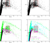 |
Fig. 4. Synthetic distributions of stars in the (J−Ks,J) diagram, obtained by assuming constant SFR and different metal-enrichments. The different panels correspond to the cases with no metal-enrichment (top left), with the metallicity gradually increasing until Z = 8 × 10⁻³ (bottom left), and Z⊙ (bottom right). The top right panel reports the results obtained with no metal-enrichment and no mass loss during the RGB phase. The different colours refer to stars with different metallicity. The grey-shaded region corresponds to the JAGB box proposed by Magnus et al. (2024). |
4.1. The case of no metal-enrichment
The first case considered is a galaxy where the metallicity of the stars formed did not change with time and remained constant at Z = 10−3. The selection of Z = 10−3 as the baseline metallicity for our simulations is primarily motivated by the fact that this value represents a realistic lower limit to the metallicities typically found in the dwarf and irregular galaxies investigated (Marconi et al. 1995; Grebel 2020; Tolstoy et al. 2009). Furthermore, the adoption of a constant SFR coupled with a “no-metal-enrichment” scenario provides a realistic approximation for many dwarf and irregular galaxies both within and outside the LG (Marconi et al. 1995; Grebel 2020; Tolstoy et al. 2009). These systems often exhibit moderate and persistent star formation activity when averaged over long timescales, resulting in a very slow chemical enrichment of the interstellar medium. For such galaxies, the change in metallicity during the critical 1–6 Gyr window is effectively negligible. This case also acts as a fundamental benchmark to isolate the impact of the SFH itself on the JLF, allowing us to assess the method’s intrinsic stability before introducing the complexities of rapid chemical evolution.
According to the results regarding the Z = 10−3 metallicity reported in Fig. 3 (see the dark green line), we deduce that the stars currently evolving in the J region formed between ∼1 Gyr and ∼6 Gyr ago. The mass (and hence age) distribution of the stars is determined by (1) whether the stars of a given mass enter the J region; (2) the time spent in the J region; (3) the duration of the epochs during which the stars entering the J region formed; and (4) the IMF of the stars formed. In the present case, point (1) restricts the analysis to the 1−2.5 M⊙ mass range. Point (2) favors the contribution of stars descending from 2−2.5 M⊙ progenitors, as shown in Fig. 3. The formation of low-mass stars is favored on the basis of points (3) and (4), given the steepening of the evolutionary time–mass relation, toward the low-mass domain. Overall, in the present case we find that ∼35% of the J population descends from 1−1.3 M⊙ progenitors, ∼30% from 1.7−2 M⊙ stars, and the remaining objects descend from stars with masses between 1.3−1.7 M⊙ and above 2 M⊙ stars.
The synthetic distribution of the stars obtained in this case is shown in the top left panel of Fig. 4, while Fig. 5 shows the JLF obtained. The region of the CMD considered is that within the 1.5 < J−KS < 2 mag color strip. Figure 5 refers to the general luminosity function (LF), with no restrictions on the J flux of the stars; the thick portion of the LF corresponds to the JLF of the stars falling within the box defined by Magnus et al. (2024), where the color constraint is complemented by the requirement that −6.83 < MJ < −5.63 mag.
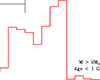 |
Fig. 5. The JLF of the stars populating the 1.5 < (J−KS < 2 mag region of the color-magnitude (J−KS,J) diagram, in a galaxy characterized by constant SFR, with metallicity Z = 10−3. The thick, red part of the histogram refers to the stars in the box suggested by Magnus et al. (2024), with −6.83 < MJ < −5.63 mag. |
The LF exhibits a prominent peak at MJ = −6.4 mag, which is due to stars descending from progenitors with masses clustered around 2 M⊙, which formed around 1 Gyr ago. The presence of this peak is consistent with the results shown in Fig. 3, indicating that these are the stars that evolve longest within the J region of the CMD. A further, subtler reason for the presence of the primary peak in the JLF is that ∼ 2 M⊙ is the upper mass limit for the occurrence of the helium flash at the metallicity Z = 10−3, and that the mass-luminosity relation flattens for the masses just below this threshold. Therefore, all stars of masses within a range of several tenths of a solar mass, centered around 2 M⊙, evolve at similar luminosities during the AGB phase, and, more specifically, they enter the J region with MJ ∼ −6.4 mag.
As discussed in the previous section, ∼ 2 M⊙ stars evolve into the J region after experiencing a few TPs following the achievement of the C star stage and remain within it during a few inter-pulse phases, during which the surface carbon and C/O ratio increase from 0.002 to 0.005 and from ∼5 to ∼10, respectively. At the same time the luminosity rises from 6500 L⊙ to 8000 L⊙. The excess of carbon relative to oxygen, which is the key quantity driving the formation of dust (Ferrarotti & Gail 2006), is on the order of (nC−nO)/nH ∼ 3−6 × 10⁻⁴, which favors the production of carbonaceous dust (essentially amorphous carbon, given the low metallicity), with rates spanning the 10−10−10−9 M⊙/yr range.
We note the steep drop in the JLF at MJ < −6.4 mag, which is within the range of J magnitudes attained by the progeny of M > 2 M⊙ stars. This is partly due to the shorter crossing timescale of the J region for these stars than for their slightly lower-mass counterparts, as shown in Fig. 3, and also to the steepening of the mass-luminosity relationship for the masses above the threshold for the occurrence of the helium flash. Indeed, the luminosities at which the stars evolve while crossing the J region are 6−8 × 10³ L⊙ for 1.7−2 M⊙, 104 L⊙ for 2.25 M⊙, 1.2 × 10⁴ L⊙ for 2.5 M⊙.
Toward the faint end of the JLF, progressively larger contributions arise from stars descending from lower-mass progenitors. The secondary peak in the figure, at MJ = −5.8 mag, is due to the progeny of 1 M⊙ < M < 1.3 M⊙ stars, which evolve within the J region with −6 < MJ < −5.7 mag. The presence of this secondary peak in the JLF is favored by the extended time interval over which these stars formed, which extends from ∼5 Gyr to ∼2 Gyr ago (point 3 above). This partly counterbalances the shorter time spent within the J region when compared to the higher-mass counterparts of the same metallicity (point 2).
Unlike the stars responsible for the primary peak in the JLF, these sources cross the J region soon after becoming C stars, with luminosities of ∼ 5000 L⊙, and they evolve rapidly toward the red side of the CMD. During this phase their surface carbon is ∼2 − 3 × 10⁻³, which corresponds to C/O ∼ 4−5 and to a carbon excess with respect to oxygen (nC−nO)/nH ∼ 2−3 × 10⁻⁴. The formation rate of carbon dust is of the order of a few 10−10M⊙/yr.
4.2. The slow metal-enrichment
We now set the assumption of constant metallicity aside and assume that the metal content of the galaxy interstellar medium increased over different timescales, τZ. At this stage we only considered mild metal-enrichment histories, where the metallicity increases up to Z = 8 × 10⁻³.
Figure 6 shows the evolution of the JLF as the timescale of the metal-enrichment becomes shorter. For clarity’s sake we limited ourselves to showing the cases of: a) no metal-enrichment, discussed earlier in this section, whose synthetic distribution on the CMD and the corresponding JLF are shown in the top left panel of Fig. 4 and in Fig. 5, respectively; b) an intermediate case in which the metallicity gradually increased, until reaching Z = 4 × 10⁻³ 4 Gyr ago, and then remained constant during the subsequent epochs; c) the case in which Z increased until Z = 4 × 10⁻³ 5 Gyr ago, reached Z = 8 × 10⁻³ 2 Gyr ago, and has since remained constant. The synthetic CMD obtained in the latter case is shown in the bottom left panel of Fig. 4.
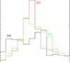 |
Fig. 6. JLF of the stars in the JAGB box defined by Magnus et al. (2024), obtained with three different assumptions regarding the metal-enrichment of the interstellar medium. (a) the same case shown in Fig. 5, where no metal-enrichment occurred; (b) the metal content of the interstellar medium increases up to Z = 4 × 10⁻³ 4 Gyr ago, and then remained unchanged, (c) Z increased until Z = 4 × 10⁻³ 5 Gyr ago, then to Z = 8 × 10⁻³ 2 Gyr ago. |
The results reported in Fig. 6 indicate that the faster the metal-enrichment of the interstellar medium, the fainter the peak of the JLF becomes; we find  in cases (a), (b), and (c) listed above, respectively. The shape of the JLF is also sensitive to the timing of the metal-enrichment. The two extreme cases are (a), in which most of the JLF is distributed at J fluxes fainter than the peak value, and (c), in which the majority of the stars populate the
  tail of the distribution; case (b) is intermediate, as the JLF is distributed around the sharp peak, located at
  mag. While
  changes, the mean J magnitude remains constant at
  mag. The metal-enrichment of the interstellar medium affects the morphology of the JLF, in such a way that we gradually move from the
  to the
  condition: the differences
  are 0.14 mag, 0 mag, ∼ − 0.14 mag in cases (a), (b), (c), respectively.
The change in the morphology of the JLF with the timing of the metal-enrichment can be understood by comparing the properties of the stars of similar masses and different metallicities, in particular in the 1 − 6 Gyr age range. Generally, if the metal-enrichment occurred earlier than ∼1 Gyr ago, the metal-poor stars descending from ∼ 2 M⊙ progenitors are replaced by their counterparts of similar mass and higher metallicity, which, as can be seen in Fig. 2, are fainter. Under these conditions the peak of the JLF is inevitably shifted to lower J fluxes. This is confirmed by the differences between the JLFs of cases (a) and (b) shown in Fig. 6, which peak at  mag and
  mag, respectively. The reason why the peak of the JLF in case (b) is sharper than in case (a) is that both ∼ 2 M⊙ stars of metallicity Z ∼ 3 − 4 × 10⁻³ and metal-poor stars of lower mass evolve at
  mag within the J region. No secondary peak is found in the JLF corresponding to case (b), because a non-negligible fraction of the metal-poor, low-mass stars, which were identified as the main contributors to the secondary peak characterizing the JLF of case (a), are replaced by their higher-metallicity counterparts, which barely enter the J region (see Fig. 3). In case (c) the peak of the JLF occurs at even fainter magnitudes than in cases (a) and (b), because the stars spending the longest time within the J region descend from 1.7−2 M⊙ progenitors of metallicity Z = 8 × 10⁻³, which are on average fainter than their lower-metallicity counterparts. In this case the primary peak at MJ = −6.1 mag is produced by a combination of the aforementioned 1.7−2 M⊙ stars of metallicity Z = 8 × 10⁻³ and ∼ 1.5 M⊙ stars of metallicity Z = 4 × 10⁻³.
4.3. Fast metal-enrichment, up to solar metallicities
We now study the shape of the JLF in cases in which the metal-enrichment proceeded at rates higher than those considered so far, up to the most extreme cases in which solar metallicity has been reached. In Fig. 7 we compare the JLF corresponding to case (c) in Fig. 6 with those obtained by assuming that the metallicity increased until reaching Z = 8 × 10⁻³ 4 Gyr ago (magenta line), and then with the two most extreme cases in which the solar metallicity was eventually reached, either 1 Gyr ago (dark green line) or 2 Gyr ago (cyan line, the corresponding synthetic CMD being shown in the bottom right panel of Fig. 4).
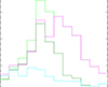 |
Fig. 7. JLF of AGB stars in the box of the CMD defined by Magnus et al. (2024), for different assumptions regarding the metal-enrichment of the interstellar medium of the galaxy. The color-coding is the following: light green shows same as case (c) in Fig. 6; magenta shows the metallicity increased up to Z = 8 × 10⁻³, 4 Gyr ago, and then constant after that; dark green shows when solar metallicity took over, 1 Gyr ago; cyan shows when solar metallicity took over, 2 Gyr ago. |
Earlier in this section we stated that the faster the metal-enrichment of the interstellar medium, the fainter the  . Figure 7 shows that this trend is reversed when even faster metal-enrichments are considered. The comparison between case (c), in which the metallicity Z = 8 × 10⁻³ was reached 2 Gyr ago, with the case where the same Z was reached during earlier epochs – i.e., 4 Gyr ago – shows that in the latter case the JLF is more distributed toward the bright side, with
  mag. This difference can be explained by comparing the slopes of the τJAGB versus mass (or time) trends shown in Fig. 3, where it is clear that the Z = 8 × 10⁻³ relation is steeper than those of the lower metallicities. Under these conditions the JAGB population is primarily composed of M ≥ 1.5 M⊙ stars, and the low-mass tail is scarcely present; therefore, the JLF peaks at the magnitudes of the brightest stars. The JLF of the case in question, shown in magenta in Fig. 7, is characterized by the presence of a secondary peak, at MJ = −6.1 mag, which is associated with M < 1.5 M⊙ stars of lower metallicity. While
  changes, the mean value is only slightly brighter than in the previous cases, with
  mag.
mag.
When the solar metallicity is reached, the framework described so far changes significantly, owing to the peculiar behavior of the stars of solar chemistry, which cross the J region much faster than the subsolar and metal-poor counterparts (see Fig. 3). If the solar metallicity was reached more recently than ∼6 Gyr ago, the population of the J region is dominated by old stars of subsolar metallicity, with a minor, if not negligible, contribution from the younger, solar-metallicity stars. In the case where solar-metallicity stars formed only during the last 1 Gyr, most of the population of the J region is composed of 1.5−2 M⊙ stars of subsolar metallicity. The corresponding JLF, shown by the dark green line in Fig. 7, peaks at −6.1 mag, and has  mag. In the case represented by the cyan line, where solar metallicity was already reached 2 Gyr ago, even the stars descending from 1.7−2 M⊙ progenitors are characterized by solar chemical composition. As shown in Fig. 3, these stars cross the J region on significantly shorter timescales than their subsolar-metallicity counterparts. Consequently, the number of objects populating the J region drops sharply, leading to a substantial decrease in the counts across the entire JLF.
4.4. The role of the mass loss during the red giant branch phase
As discussed in Sect. 2, the results presented in this section are based on the assumption that low-mass stars experienced mass loss during the RGB evolution, such that on average the mass of the envelope was reduced by 0.2 M⊙ by the time they reached the TRGB. The role of RGB mass loss in the AGB evolution can be understood by noting that stars losing mass during the ascent of the RGB start the core helium-burning phase and the subsequent AGB evolution with a smaller envelope mass: the AGB phase is consequently shorter, since the envelope is lost after the star experiences fewer TPs than in the absence of RGB mass loss. This is mostly relevant for low-mass stars with M < 1.5 M⊙, because these sources evolve longer through the RGB and therefore suffer larger mass loss than their more massive counterparts; even a few tenths of solar masses lost represents a significant fraction of the total mass of the envelope.
The RGB mass loss inevitably affects the numerical consistency and the luminosity distribution of the stars populating the J region, since low-mass stars enter the J region soon after becoming C stars. As this condition requires the occurrence of several TDU events, strong RGB mass loss prevents low-mass stars from reaching the J region, which would then be populated only by stars descending from progenitors of mass above solar, so the JLF would be shifted toward the brighter J magnitudes.
To understand the role played by the assumptions regarding the RGB mass loss on the results obtained by the present analysis, we reconsider some of the cases discussed in the previous sections. We repeated the simulations based on the population synthesis approach described in Sect. 2, assuming that low-mass stars experienced no mass loss during the RGB phase. In particular, we addressed the case of no metal-enrichment (presented in Fig. 5), the case with mild metal-enrichment, in which the metallicity of the interstellar medium increased up to Z = 4 × 10⁻³ 4 Gyr ago (the one represented in red in Fig. 6), and the case in which the metallicity increased until reaching Z = 8 × 10⁻³ 4 Gyr ago (presented in magenta in Fig. 7).
Figure 8 presents a comparison between the results obtained under the standard assumption of δmRGB = 0.2 M⊙ and those obtained with no RGB mass loss for the three cases considered. In the no-metal-enrichment case, the synthetic distribution of the stars on the CMD obtained in the case where no mass loss took place during the RGB evolution is reported in the top right panel of Fig. 4. The corresponding JLF, shown in the left panel of Fig. 8, exhibits a primary peak at MJ ∼ −5.85 mag, which is significantly fainter than the peak found in the standard case located at MJ ∼ −6.4 mag. This difference is due to the evolution of stars descending from 0.9−1 M⊙ progenitors, formed between 9 and 6 Gyr ago. These stars evolve into the J region if δmRGB = 0, whereas if their envelope is eroded by the RGB mass loss they fail to become C stars, and thus evolve along the blue side of the CMD without entering the J region. These stars outnumber the higher-mass counterparts because of the shape of the IMF, which favors the presence of the stars of lower masses, and, more importantly, the duration of the time over which they formed, which extends over ∼3 Gyr.
 |
Fig. 8. Comparison between the JLF obtained by assuming an average RGB mass loss of 0.2 M⊙ (solid track) with those obtained by assuming that no mass loss occurred during the RGB phases. The cases presented are the following: no metal-enrichment and constant metallicity Z = 10−3 (left panel), and metal-enrichment up to Z = 4 × 10⁻³ (middle panel) and Z = 8 × 10⁻³ (right panel). |
The JLF of the galaxy is heavily affected by the assumptions regarding the RGB mass loss even in the case where some metal-enrichment occurred, such as the second one considered here. This can be seen in the middle panel of Fig. 8, where the sharp distribution around the peak at MJ ∼ −6.3 mag, found in the standard case, is replaced by a double-peaked distribution, in which the primary peak, similarly to the previous case, is at MJ ∼ −5.85 mag. This result is not surprising, considering that the old population of the galaxy is still made up of low-mass, metal-poor stars, for which the same arguments exposed previously hold. The primary peak of the JLF is once more due to the presence of the progeny of 0.9−1 M⊙ stars, which have just reached the C star stage while evolving within the J region.
We finally considered a case of an earlier metal-enrichment, which led to the formation of Z = 8 × 10⁻³ stars during the period extending from 4 Gyr ago to the present day. In this case, as shown in the right panel of Fig. 8, the change in the JLF is less dramatic than in the two previous examples, because the location of the primary peak only changes by 0.1 mag if the RGB mass loss is neglected. However, there remain notable differences, particularly in the general shape of the JLF, which is more biased toward the faint side when no RGB mass loss is considered. This faint tail of the JLF is due to the presence of low-mass, metal-poor stars, formed ∼8 Gyr ago, that populate the J region.
These findings show that if the mass loss suffered by low-mass stars during the RGB phase is neglected, the results presented earlier in this section would require substantial revision, particularly in the cases of slow metal-enrichment. Indeed, the mean J magnitude of the JAGB population would be  mag (to be compared with the
  mag values found before), which reflects the shift of the entire JLF to the faint side. When a faster metal-enrichment is considered, only part of the metal-poor, low-mass stars enter the J region, so
  mag, which is more similar to the values obtained by assuming δmRGB = 0.2 M⊙.
While it is important to warn the reader of this source of uncertainty, we believe that conclusions drawn in the previous sections are substantially robust, since the mass loss suffered by stars evolving through the RGB phase is a consolidated result of the studies of the stellar populations. Besides the aforementioned investigations on globular clusters, we mention, for example, the recent study of the evolved stellar population of Andromeda, by Gavetti et al. (2025), which demonstrated that full consistency between the results from synthetic modeling and the observed distribution of the stars along the CMD built with HST filters is obtained only if we assume that low-mass stars suffer average mass loss of 0.2 M⊙ during the RGB evolution. The same conclusion was reached by Ventura et al. (2026) in a study focused on the statistics of RGB and AGB stars in metal-poor dwarf and irregular galaxies.
5. Discussion
The study of the AGB population of the J region of the CMD is crucial to assessing whether these stars can be used as distance indicators. This is only possible if we can identify at least some of the properties of their LF that are independent of the previous history of the galaxies considered. This is a necessary condition for a general application of this method, which would otherwise be restricted to the galaxies for which the SFH was deduced on the basis of independent investigations. In this regard, both the mean and the peak J magnitude of JAGB stars have been investigated as possible candidates for an independent and robust estimate of galaxy distances (Lee 2023; Lee et al. 2024, 2025; Li et al. 2024, 2025).
The results presented and discussed in the previous section outlined the important role played by the rate of metal-enrichment of the interstellar medium in determining the JLF of the stars populating the J region of a given galaxy. The timing of the metal-enrichment was shown to affect not only the primary parameters of the JLF, such as the peak J magnitude, but more generally the shape of the distribution and the details of how the JLF declines toward the fainter and the brighter ends.
Before entering the discussion regarding the sensitivity of the peak and mean J magnitudes of the stars in the J region to the timing of the metal-enrichment of the interstellar medium, we deem it important to underline that both quantities are substantially independent of the vertical extension (in magnitude) of the JAGB box. This is obvious for  , as in all the cases investigated in the previous section we found that it definitely falls within the ( − 6.35 : −6.1) mag range. On the other hand, even
  would be scarcely affected by the size of the JAGB box. If the box extends brighter than the upper limit proposed by Magnus et al. (2024), it is possible that massive AGB stars of mass M ≥ 3 M⊙ enter the J region while experiencing HBB. This would contaminate the J region with oxygen-rich objects, but their evolutionary times are so short that only a few of them are expected to be counted, so the estimated mean J magnitude would be practically unchanged. This is confirmed by the various cases examined in Sect. 4 (presented in Figs. 5, 6, and 7), where it is clear that there is a significant drop in the JLF on the bright side of the distribution. Even if the lower limit of the JAGB box were extended to fainter magnitudes than suggested by Magnus et al. (2024),
  would be barely affected. In this case the stellar population in the J region would indeed remain substantially unchanged, because the stars of masses below ∼ 0.9 M⊙, which during the AGB phase evolve at MJ > −5.7 mag, do not produce dust; thus, the corresponding evolutionary tracks remain on the blue side of the CMD, never entering the JAGB box.
A summary of the results obtained by the various simulations done in the present work is reported in Fig. 9, showing how the skewness and  of the JLF vary as a function of
  , the difference between the peak and the average MJ value. In both planes the curves trace counterclockwise trajectories, starting from the case where no metal-enrichment occurred (Fig. 5) and ending with the case where the Z = 8 × 10⁻³ metallicity was reached 4 Gyr ago (magenta line in Fig. 7).
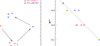 |
Fig. 9. Skewness (left panel) and peak J magnitude (right panel) of JLFs of the synthetic stellar populations of the J region of the (J−KS,J) diagram, as a function of the difference between the mean and the peak J magnitudes. The various points refer to results obtained with different assumptions regarding the metal-enrichment, including the case where no metal-enrichment occurred (black triangle), a few cases where the final metallicity of the galaxy grew to Z = 4 × 10⁻³ (red triangles), and some simulations where the final metallicity of the interstellar medium is Z = 8 × 10⁻³. |
The initial part of the trends shown in Fig. 9 extends from the metal-poor galaxy that experienced no metal-enrichment, discussed in Sect. 4.1, to the case where the metallicity of the interstellar medium reached Z = 8 × 10⁻³ 2 Gyr ago, shown in light green in Figs. 6 and 7. In these cases the main factor affecting the change in the JLF, discussed in Sect. 4, is that higher-metallicity stars evolve at fainter luminosities than the lower-metallicity counterparts of similar mass, so that the peak of the JLF occurs at fainter J fluxes as the metal-enrichment becomes faster; this is the reason why  increases from ∼ − 0.15 mag to 0.15 mag, while
  changes from –6.4 mag to –6.1 mag. The shape of the JLF is also sensitive to the metal-enrichment, as witnessed by the change in the skewness of the distribution. Initially, the JLF (see Fig. 5) is mainly distributed on the bright side; thus, the skewness is positive and equal to ∼0.2. Metal-enrichment leads to increasingly asymmetric JLFs skewed toward fainter J magnitudes (see Fig. 6), and the skewness eventually reaches values as low as ∼ − 0.3. The most extreme case, in which the metallicity reaches Z = 8 × 10⁻³, is the only exception to this trend, since the distribution becomes more symmetric; thus, the skewness is approximately null.
Both the trends reported in Fig. 9 are seen to reverse at  mag. From this point the most relevant factor for the shape of the JLF is that low-mass stars of metallicity Z ≥ 8 × 10⁻³ barely enter the J region; thus, the JLF is determined by the progeny of M ≥ 1.5 M⊙ stars only, which causes the LF to move toward the bright J magnitudes again.
  decreases to –6.3 mag, while
  decreases down to ∼ − 0.05 mag, and the skewness of the distribution becomes positive again. However, the values are small, i.e., on the order of 0.05.
These results indicate that the mean J magnitude of the JAGB population is practically unaffected by the details of the metal-enrichment of the galaxy and is equal to  mag, with an uncertainty limited to 0.05 mag. In the majority of cases the peak J magnitude of the distribution is also
  mag, except for a few cases, in which it changes by ∼0.15 mag. We note that the data collected so far – obtained in particular from the massive compilations presented by Freedman & Madore (2020) and Freedman et al. (2025) – seem to rule out the occurrence of such extreme cases, pointing in favor of a universal Gaussian distribution peaking at ∼ − 6.2 mag. In the evaluation of the quality of
  and
and  as distance indicators of galaxies, it is important to note that while the mean J magnitude appears more stable and less sensitive to the metal-enrichment of the galaxies,
  has the advantage of being unaffected by possible contamination from, for example, unresolved, red-background galaxies, or even faint objects, erroneously scattered into the color range of the JAGB stars.
The above arguments indicate that the peak J magnitude of the JLF cannot be considered as a reliable distance indicator, because it is sensitive to differences in the metal-enrichment histories of galaxies, varying by up to 0.3 mag. On the other hand, it is remarkable that the changes in  are accompanied by variations in the general shape of the JLF, in such a way that the mean J magnitude of the JAGB population is almost unaffected by the details of the metal-enrichment. The magnitude is equal to
  mag, with an uncertainty limited to 0.05 mag.
The use of the J method to estimate distances in galaxies that experienced very rapid metal-enrichment, eventually reaching solar metallicity, is problematic. The reason is that the evolutionary timescales of these objects become extremely short after they become C stars, so the crossings through the J region of the CMD are very fast. If the metal-enrichment was so fast that the solar metallicity was reached earlier than ∼2 Gyr ago, the contribution from solar-metallicity stars to the JAGB population would become negligible because of their extremely short crossing times through the J region. Under these conditions, the J region would be populated predominantly by older, lower-metallicity stars, and the statistical properties discussed above would no longer apply.
6. Conclusions
We used population synthesis results to investigate the applicability of the J method to derive the distances of galaxies. We assumed a constant SFR from galaxy formation to the present and we focused on the effects of the timing of interstellar medium enrichment on the shape of the JLF for the stars in the J region of the CMD.
The stars currently populating the J region descend from progenitors with masses in the 1−3 M⊙ range, which formed during the epochs spanning from ∼6 Gyr to ∼1 Gyr ago. Older stars than ∼6 Gyr barely enter the J region, whereas the stars younger than ∼1 Gyr evolve brighter than the upper limit of the box selected to define the J region, and in any case their crossing times would be too short to significantly affect the statistics. The progeny of 2−2.5 M⊙ stars provides the most relevant contribution to the JAGB population, because they evolve within the J region for longer timescales than both their lower-mass counterparts.
The shape of the JLF turns out to be extremely sensitive to the timing of the metal-enrichment of the galaxy, owing to the differences in the evolutionary properties of stars of similar masses and different metallicities. This particularly concerns the time evolution of the luminosity and the time when the C star stage is reached, both of which are relevant for the shape of the JLF and the peak of the distribution of the J magnitudes of the stars in the J region.
The peak J magnitude of the JLF cannot be used to infer the distance of galaxies, because it is extremely sensitive to the metal-enrichment process, and changes by 0.3 mag, spanning the range from  mag to
  mag. On the other hand, the mean J magnitude turns out to be a much more robust distance indicator, as it is found to be
  mag, independently of the timing of the metal-enrichment process.
The applicability of the method to the galaxies where the metal-enrichment was so fast that solar-metallicity stars formed more than ∼2 Gyr is questionable; this is because these stars evolve very quickly during the evolutionary phases following the achievement of the C star stage, so their transit across the J region of the CMD is extremely rapid.
The applicability of the J method to measure distances must be further tested against variations in the SFR, which alter the relative fractions of stars of different age and mass and may consequently affect the mass and luminosity distribution of the stars populating the J region.
References
- Aoyama, S., Hou, K.-C., Hirashita, H., Nagamine, K., & Shimizu, I. 2018, MNRAS, 478, 4905 [NASA ADS] [CrossRef] [Google Scholar]
- Blöcker, T., & Schönberner, D. 1991, A&A, 244, L43 [Google Scholar]
- Bortolini, G., Östlin, G., Habel, N., et al. 2024, A&A, 689, A146 [NASA ADS] [CrossRef] [EDP Sciences] [Google Scholar]
- Bortolini, G., Correnti, M., Adamo, A., et al. 2025, ApJ, 991, 212 [Google Scholar]
- Calura, F., Matteucci, F., & Menci, N. 2004, MNRAS, 353, 500 [Google Scholar]
- Conroy, C. 2013, ARA&A, 51, 393 [NASA ADS] [CrossRef] [Google Scholar]
- Correnti, M., Bortolini, G., Dell’Agli, F., et al. 2025, ApJ, 990, 72 [Google Scholar]
- Dell’Agli, F., Ventura, P., Garcia Hernandez, D. A., et al. 2014b, MNRAS, 442, L38 [Google Scholar]
- Dell’Agli, F., García-Hernández, D. A., Rossi, C., et al. 2014a, MNRAS, 441, 1115 [Google Scholar]
- Dell’Agli, F., Ventura, P., Schneider, R., et al. 2015a, MNRAS, 447, 2992 [Google Scholar]
- Dell’Agli, F., García-Hernández, D. A., Ventura, P., et al. 2015b, MNRAS, 454, 4235 [Google Scholar]
- Dell’Agli, F., Di Criscienzo, M., Boyer, M. L., et al. 2016, MNRAS, 460, 4230 [Google Scholar]
- Dell’Agli, F., Di Criscienzo, M., Ventura, P., et al. 2018, MNRAS, 479, 5035 [Google Scholar]
- Dell’Agli, F., Di Criscienzo, M., García-Hernández, D. A., et al. 2019, MNRAS, 482, 4733 [Google Scholar]
- Diemer, B., Sparre, M., Abramson, L., & Torrey, P. 2017, ApJ, 839, 26 [Google Scholar]
- Ferrarotti, A. S., & Gail, H.-P. 2002, A&A, 382, 256 [NASA ADS] [CrossRef] [EDP Sciences] [Google Scholar]
- Ferrarotti, A. S., & Gail, H.-P. 2006, A&A, 447, 553 [CrossRef] [EDP Sciences] [Google Scholar]
- Freedman, W. L., & Madore, B. F. 2020, ApJ, 899, 67 [NASA ADS] [CrossRef] [Google Scholar]
- Freedman, W. L., Madore, B. F., Hoyt, T. J., et al. 2025, ApJ, 985, 203 [Google Scholar]
- Gavetti, C., Ventura, P., Dell’Agli, F., et al. 2025, A&A, 699, A23 [NASA ADS] [CrossRef] [EDP Sciences] [Google Scholar]
- Gavetti, C., Ventura, P., Dell’Agli, F., et al. 2026, A&A, 707, A384 [NASA ADS] [CrossRef] [EDP Sciences] [Google Scholar]
- Ginolfi, M., Graziani, L., Schneider, R., et al. 2018, MNRAS, 478, 4905 [NASA ADS] [CrossRef] [Google Scholar]
- Graziani, L., Schneider, R., Ginolfi, M., et al. 2015, MNRAS, 494, 1071 [Google Scholar]
- Grebel, E. K. 2020, ESA Spec. Publ., 445, 87 [Google Scholar]
- Harmsen, B., Bell, E. F., D’Souza, R., et al. 2023, MNRAS, 525, 449 [Google Scholar]
- Jegatheesan, K., et al. 2025, A&A, 694, 224 [Google Scholar]
- Kamath, D., Dell’Agli, F., Ventura, P., et al. 2023, MNRAS, 519, 2169 [Google Scholar]
- Kobayashi, C., Karakas, A. I., & Lugaro, M. 2020, ApJ, 900, 179 [Google Scholar]
- Kroupa, P. 2001, MNRAS, 322, 231 [NASA ADS] [CrossRef] [Google Scholar]
- Lee, A. J. 2023, ApJ, 956, 15 [Google Scholar]
- Lee, A. J., Freedman, W. L., Jang, I. S., Madore, B. F., & Owens, K. A. 2024, ApJ, 961, 132 [Google Scholar]
- Lee, A. J., Weisz, D. R., Ren, Y., Savino, A., & Dolphin, A. E. 2024, ArXiv e-prints [arXiv:2410.09256] [Google Scholar]
- Lee, A. J., Freedman, W. L., Madore, B. F., et al. 2025, ApJ, 985, 182 [Google Scholar]
- Li, S., Riess, A. G., Casertano, S., et al. 2024, ApJ, 966, 20 [NASA ADS] [CrossRef] [Google Scholar]
- Li, S., Riess, A. G., Scolnic, D., Casertano, S., & Anand, G. S. 2025, ApJ, 988, 97 [Google Scholar]
- Madau, P., & Dickinson, M. 2014, ARA&A, 52, 415 [Google Scholar]
- Madore, B. F., & Freedman, W. L. 2020, ApJ, 899, 66 [NASA ADS] [CrossRef] [Google Scholar]
- Magnus, E., Groenewegen, M. A. T., Girardi, L., et al. 2024, A&A, 691, A350 [NASA ADS] [CrossRef] [EDP Sciences] [Google Scholar]
- Mancini, M., Schneider, R., Graziani, L., et al. 2015, MNRAS, 451, L70 [CrossRef] [Google Scholar]
- Marconi, G., Tosi, M., Greggio, L., & Focardi, P. 1995, AJ, 109, 173 [Google Scholar]
- Marigo, P. 2002, A&A, 387, 507 [NASA ADS] [CrossRef] [EDP Sciences] [Google Scholar]
- Marini, E., Dell’Agli, F., Groenewegen, M. A. T., et al. 2021, A&A, 647, A69 [NASA ADS] [CrossRef] [EDP Sciences] [Google Scholar]
- Mazzitelli, I. 1979, A&A, 79, 251 [Google Scholar]
- Nanni, A., Bressan, A., Marigo, P., et al. 2013, MNRAS, 434, 2390 [NASA ADS] [CrossRef] [Google Scholar]
- Nanni, A., Bressan, A., Marigo, P., et al. 2014, MNRAS, 438, 2328 [NASA ADS] [CrossRef] [Google Scholar]
- Nanni, A., Marigo, P., Groenewegen, M. A. T., et al. 2016, MNRAS, 462, 1215 [NASA ADS] [CrossRef] [Google Scholar]
- Nanni, A., Marigo, P., Girardi, L., et al. 2018, MNRAS, 473, 5492 [NASA ADS] [CrossRef] [Google Scholar]
- Nanni, A., Groenewegen, M. A. T., Aringer, B., et al. 2019, MNRAS, 487, 502 [NASA ADS] [CrossRef] [Google Scholar]
- Nenkova, M., Ivezic, Z., & Elitzur, M. 1999, Thermal Emission Spectroscopy and Analysis of Dust, Disks, and Regoliths, 20 [Google Scholar]
- Nikolaev, S., & Weinberg, M. D. 2000, ApJ, 542, 804 [NASA ADS] [CrossRef] [Google Scholar]
- Pacifici, C., Kassin, S., Weiner, B., et al. 2016, ApJ, 832, 79 [Google Scholar]
- Ripoche, P., Heyl, J., Parada, J., et al. 2020, MNRAS, 495, 2858 [NASA ADS] [CrossRef] [Google Scholar]
- Rogers, B., Ferreras, I., et al. 2010, MNRAS, 402, 447 [Google Scholar]
- Romano, D. 2022, A&ARv, 30, 7 [NASA ADS] [CrossRef] [Google Scholar]
- Sackmann, I.-J., & Boothroyd, A. I. 1992, ApJ, 392, L71 [NASA ADS] [CrossRef] [Google Scholar]
- Schneider, R., & Maiolino, R. 2024, A&ARv, 32, 2 [NASA ADS] [CrossRef] [Google Scholar]
- Tailo, M., Milone, A. P., Lagioia, E. P., et al. 2021, MNRAS, 503, 694 [NASA ADS] [CrossRef] [Google Scholar]
- Tolstoy, E., Hill, V., & Tosi, M. 2009, ARAA, 47, 371 [CrossRef] [Google Scholar]
- Valiante, R., Schneider, R., Bianchi, S., et al. 2009, MNRAS, 397, 1661 [CrossRef] [Google Scholar]
- Valiante, R., Schneider, R., Salvadori, S., et al. 2011, MNRAS, 416, 1916 [Google Scholar]
- Ventura, P., Zeppieri, A., Mazzitelli, I., & D’Antona, F. 1998, A&A, 334, 953 [Google Scholar]
- Ventura, P., D’Antona, F., Mazzitelli, I., et al. 2001, ApJ, 550, L65 [Google Scholar]
- Ventura, P., Di Criscienzo, M., Schneider, R., et al. 2012, MNRAS, 420, 1442 [Google Scholar]
- Ventura, P., Dell’Agli, F., Schneider, R., et al. 2014, MNRAS, 439, 977 [NASA ADS] [CrossRef] [Google Scholar]
- Ventura, P., Karakas, A., Dell’Agli, F., et al. 2018, MNRAS, 475, 2282 [NASA ADS] [Google Scholar]
- Ventura, P., Dell’Agli, F., Tailo, M., et al. 2022, Universe, 8, 45 [NASA ADS] [CrossRef] [Google Scholar]
- Ventura, P., D’Souza, R., Dell’Agli, F., et al. 2026, A&A, 709, A219 [NASA ADS] [CrossRef] [EDP Sciences] [Google Scholar]
- Wood, P. R., Kamath, D., & Van Winckel, H. 2013, MNRAS, 435, 355 [Google Scholar]
The achievement of the C/O > 1 condition is per se not sufficient with regard to the formation of carbon dust, because the CO molecules are very stable, thus only the carbon in excess of oxygen is available to condense into solid particles (Ferrarotti & Gail 2006).
All Figures
|
Fig. 1. Time variation of the surface C/O ratio of model stars of metallicity Z = 10−3 (black lines), Z = 4 × 10⁻³ (blue), and Z = 0.014 (green) that formed ∼1 Gyr ago (left panel), ∼3 Gyr ago (middle), and ∼5 Gyr ago (right). The magenta portion of the lines indicates the phases during which the model stars cross the J region. The horizontal gray lines indicate the time when the stars become C stars. Times are counted from the beginning of the TP–AGB phase. The masses reported in the middle and right panels refer to the start of the core helium-burning phase. |
| In the text | |
|
Fig. 2. Evolutionary tracks of stars of different masses and metallicities in the color–magnitude (J−KS,J) diagram. For M≤ 2 M⊙ the masses were taken at the beginning of the core helium-burning phase. The points along each track refer to the phases of maximum luminosity experienced during an inter-pulse phase. Open symbols refer to the phases during which the star is O-rich, whereas full points indicate C-rich phases. The gray shaded box indicates the J region defined by Magnus et al. (2024). |
| In the text | |
|
Fig. 3. Times spent within the J region by model stars of different masses and metallicities as a function of the progenitor’s mass (left panel) and of the formation epoch (right). The masses for M ≤ 2 M⊙ stars refer to the start of the core helium-burning phase. For masses below 1.5 M⊙ we considered an average mass loss during the RGB evolution of 0.2 M⊙; thus, the formation epochs reported on the abscissa of the right panel refer to those of the model stars of mass 0.2 M⊙ higher than those reported on the abscissa of the left panel. Each sequence is limited to the masses whose evolutionary tracks enter the J region. |
| In the text | |
|
Fig. 4. Synthetic distributions of stars in the (J−Ks,J) diagram, obtained by assuming constant SFR and different metal-enrichments. The different panels correspond to the cases with no metal-enrichment (top left), with the metallicity gradually increasing until Z = 8 × 10⁻³ (bottom left), and Z⊙ (bottom right). The top right panel reports the results obtained with no metal-enrichment and no mass loss during the RGB phase. The different colours refer to stars with different metallicity. The grey-shaded region corresponds to the JAGB box proposed by Magnus et al. (2024). |
| In the text | |
|
Fig. 5. The JLF of the stars populating the 1.5 < (J−KS < 2 mag region of the color-magnitude (J−KS,J) diagram, in a galaxy characterized by constant SFR, with metallicity Z = 10−3. The thick, red part of the histogram refers to the stars in the box suggested by Magnus et al. (2024), with −6.83 < MJ < −5.63 mag. |
| In the text | |
|
Fig. 6. JLF of the stars in the JAGB box defined by Magnus et al. (2024), obtained with three different assumptions regarding the metal-enrichment of the interstellar medium. (a) the same case shown in Fig. 5, where no metal-enrichment occurred; (b) the metal content of the interstellar medium increases up to Z = 4 × 10⁻³ 4 Gyr ago, and then remained unchanged, (c) Z increased until Z = 4 × 10⁻³ 5 Gyr ago, then to Z = 8 × 10⁻³ 2 Gyr ago. |
| In the text | |
|
Fig. 7. JLF of AGB stars in the box of the CMD defined by Magnus et al. (2024), for different assumptions regarding the metal-enrichment of the interstellar medium of the galaxy. The color-coding is the following: light green shows same as case (c) in Fig. 6; magenta shows the metallicity increased up to Z = 8 × 10⁻³, 4 Gyr ago, and then constant after that; dark green shows when solar metallicity took over, 1 Gyr ago; cyan shows when solar metallicity took over, 2 Gyr ago. |
| In the text | |
|
Fig. 8. Comparison between the JLF obtained by assuming an average RGB mass loss of 0.2 M⊙ (solid track) with those obtained by assuming that no mass loss occurred during the RGB phases. The cases presented are the following: no metal-enrichment and constant metallicity Z = 10−3 (left panel), and metal-enrichment up to Z = 4 × 10⁻³ (middle panel) and Z = 8 × 10⁻³ (right panel). |
| In the text | |
|
Fig. 9. Skewness (left panel) and peak J magnitude (right panel) of JLFs of the synthetic stellar populations of the J region of the (J−KS,J) diagram, as a function of the difference between the mean and the peak J magnitudes. The various points refer to results obtained with different assumptions regarding the metal-enrichment, including the case where no metal-enrichment occurred (black triangle), a few cases where the final metallicity of the galaxy grew to Z = 4 × 10⁻³ (red triangles), and some simulations where the final metallicity of the interstellar medium is Z = 8 × 10⁻³. |
| In the text | |
Current usage metrics show cumulative count of Article Views (full-text article views including HTML views, PDF and ePub downloads, according to the available data) and Abstracts Views on Vision4Press platform.
Data correspond to usage on the plateform after 2015. The current usage metrics is available 48-96 hours after online publication and is updated daily on week days.
Initial download of the metrics may take a while.