


| Issue |
A&A
Volume 711, July 2026
|
|
|---|---|---|
| Article Number | A305 | |
| Number of page(s) | 20 | |
| Section | Stellar atmospheres | |
| DOI | https://doi.org/10.1051/0004-6361/202660113 | |
| Published online | 24 July 2026 | |
Analysis of far-infrared fine-structure emissions from the red supergiant µ Cephei
1
Max-Planck-Institut für Radioastronomie,
Auf dem Hügel 69,
53121
Bonn,
Germany
2
Laboratoire d’astrophysique de Bordeaux, Univ. Bordeaux,
CNRS, B18N, allée Geoffroy Saint-Hilaire,
33615
Pessac,
France
3
Instituto de Física Fundamental,
CSIC, C/ Serrano123,
28006
Madrid,
Spain
4
Center for Astrophysics and Space Astronomy, University of Colorado Boulder,
389 UCB,
Boulder,
CO
80309,
USA
★ Corresponding author: This email address is being protected from spambots. You need JavaScript enabled to view it.
Received:
23
March
2026
Accepted:
11
June
2026
Abstract
Context. The complex structure and dynamics of red supergiant stars (RSGs) and their variability hinder the spectral analysis of the conditions above their photosphere. RSGs share these features with their lower-mass equivalents on the asymptotic giant branch, but they are less well understood. Since RSGs are the direct progenitors of core collapse (Type II) supernovae, a better characterization is desirable.
Aims. This work aims to create a concordant model unifying stellar parameters, elemental abundances, and chromospheric properties of µ Cephei, which is among the most luminous RSGs of the Galaxy. Its distance is weakly constrained (reported values range between 390 and 870 pc), and the immediate vicinity of the photosphere is still largely uncharted territory.
Methods. For this purpose, we conducted high-resolution spectroscopy of the transparent far-infrared fine-structure line emissions from the electronic ground states of O I, C II, S I, and Fe II, with the EXES and GREAT instruments flown aboard the Stratospheric Observatory for Infrared Astronomy (SOFIA). Line-area ratios were compared with predictions from a grid of model chromospheres around an early-M-type RSG. We used a distance of 421−42+57 pc, obtained by linking spectroscopic estimators for µ Cephei to its nearinfrared interferometry, which are both available in the literature. The uptake of the observed species by the thermal-equilibrium chemistry in the inner circumstellar envelope was modeled including 523 gaseous and 190 solid species. We applied a dedicated code for the mixed radiative transfer of spectral-line and continuum emissions. The underlying opacities were obtained from statistical-equilibrium calculations and a two-component dust model comprised of silicate and alumina. The velocity structure required to match the observed line profiles accounts for bulk motions and turbulence in the stellar wind, and for the onset of a radiation-pressure-driven wind at the dust condensation zone.
Results. We identify two solutions differing in chromospheric temperature and density. The resulting thermal pressures are within a factor of four. For a clumpy medium, these models reproduce the measured line fluxes, but they require an additional source for the C II abundance, which is most likely the photo-chemistry of carbon. It is driven by far-UV emissions from shocks forming in response to, for example, encounters of outflowing and inflowing gas. A self-consistent model calls for more accurate elemental abundances at the stellar surface. For the other species, the corrections are smaller. Our models also reproduce the H I λ 21 cm flux from the recent literature.
Key words: stars: atmospheres / stars: chromospheres / circumstellar matter / stars: late-type / supergiants / stars: winds, outflows
© The Authors 2026
 Open Access article, published by EDP Sciences, under the terms of the Creative Commons Attribution License (https://creativecommons.org/licenses/by/4.0), which permits unrestricted use, distribution, and reproduction in any medium, provided the original work is properly cited.
This article is published in open access under the Subscribe to Open model.
Open Access funding provided by Max Planck Society.
1 Introduction
The mass loss from red supergiant stars (RSGs) was recognized shortly after the discovery (Biermann 1951) and explanation (Parker 1958) of the solar wind, by Deutsch (1956) and Weymann (1962), toward α Herculis and α Orionis, respectively, followed by Bernat (1977, including α Scorpii and µ Cephei). Later, inhomogeneities were found in the wind of µ Cephei and attributed to episodic mass-loss events (Mauron 1997). However, our knowledge of the extended photospheres of RSGs is still limited (Höfner & Olofsson 2018; Decin 2021). In particular, the mechanisms driving their mass loss and the dynamical role of circumstellar dust are still under debate, while they are generally understood in asymptotic giant-branch stars (AGBs), their low-mass equivalents. The great dimming of α Orionis (Betelgeuse, Guinan et al. 2020) constitutes a recent and spectacular demonstration of this uncertainty. Montargès et al. (2021) propose that a large, cold convection cell, aided by the brightness minimum of the stellar pulsation, cooled the gas locally. Its subsequent and quick condensation into dust created the veil observed in the southern hemisphere of the star. On the other hand, Harper et al. (2020b) conclude from long-term photometry that the dimming could be produced by a drop in the photospheric temperature of at least 250 K, without introducing the extinction of a recently formed dust component, for which λ25 µm spectra from the Stratospheric Observatory for Infrared Astronomy (SOFIA) show no evidence either (Harper et al. 2020a). Thereupon, several attempts were made to better constrain the evolutionary status of Betelgeuse, involving seismic models (Saio et al. 2023; challenged by Molnár et al. 2023) and a stellar companion (Dupree & Montargès 2025; Dupree et al. 2026, further references therein). While the issue is still open, the importance of this debate is emphasized by the fact that RSGs are the direct precursors of core-collapse (Type II) supernovae (SNe). The progenitor stars of the latter, if detected, rarely exceed masses above 18 M⊙ (Smartt 2015; Anderson et al. 2018), which contrasts with stellar evolution models predicting an upper limit of 30 M⊙ (Smartt 2009). This RSG problem was recently shown to be statistically significant (Rodríguez 2022), although no consensus has been reached yet (Davies & Beasor 2018, 2020b; Kochanek 2020; Davies & Beasor 2020a), which is not an ideal situation: Since Type II SNe enrich the interstellar medium (ISM) of a galaxy with pristine nucleosynthesis products, understanding their characteristics and those of their progenitors is indispensable for completing our picture of the baryon cycle.
Another underexplored and related terrain is the transition between the photospheres of RSGs and the inner boundary of their molecular circumstellar envelopes. Unlike the lower-mass AGBs, RSGs do not undergo a third dredge-up that would mix the carbon synthesized in the He-burning core via the 3α process into their convective envelopes. The extended photospheres of RSGs are thus oxygen-rich. While this is a prerequisite for SiO masers to form, observations of the latter exist only for a few objects: µ Cephei (Herschel’s “garnet star”) which is introduced below, VX Sgr (Moran et al. 1979; Su et al. 2012) for which Tabernero et al. (2021) gave evidence that it could be an extreme AGB star rather than a RSG strictly speaking, NML Cyg (Boboltz & Marvel 2000; Zhang et al. 2012b, Very Long Baseline Array observations), and VY CMa (Shibata et al. 2004; Zhang et al. 2012a; Richter et al. 2013). The two latter objects are red hypergiants, yet their masses are uncertain: For NML Cyg, estimates vary between 20–25 M⊙ (Zubko et al. 2004; Zhang et al. 2012b) and 40 M⊙ (Schuster et al. 2009), and between 8 and 25 M⊙ for VY CMa (Monnier et al. 2000; Zubko et al. 2004, respectively). The lower end of these mass ranges represents the cutoff for a SN to occur; the upper end is thought to end in a faint SN that is difficult to detect (Smartt 2009).
In contrast, the nature of µ Cephei is better constrained by a new simulation of evolutionary tracks (Ekström et al. 2012) and the estimation of its associated stellar parameters (Montargès et al. 2019), including an initial mass of 15– 20 M⊙ and a photospheric temperature of Teff = 3600 ± 140 K. This means that µ Cephei, which has no known binary companion, is a true Type II SN progenitor. It is also possible to infer the He-burning core mass from the stellar luminosity (i.e., without matching evolutionary tracks, Farrell et al. 2020b). Very long baseline interferometry (VLBI) observations of the λ7 mm SiO maser emissions from µ Cephei exist (Miyoshi et al. 1992; Colomer et al. 1992; Colomer 1993; Imai et al. 2001), but they only allow for an incomplete characterization of the gas layer overlying the photosphere. In this context, we also note that the non-detection of SiO masers in the otherwise archetypal Betelgeuse (Lambert & Vanden Bout 1978) calls for another observational approach. In this context, observations with Atacama Large Millimeter/submillimeter Array of high-excited H2O and OH lines from three RSGs were recently used as a complementary tool to analyze their extended photospheres (Baudry et al. 2023).
Far-infrared atomic fine-structure lines are therefore quite instructive, as demonstrated by Harper et al. (2021) for the case of Betelgeuse during its great dimming. These lines connect states of the same parity and in this work they arise from magnetic-dipole transitions within the electronic ground state. On the sightline to the photosphere, the [O I] 3P1 → 3P2 line at λ 63.2 µm is only moderately affected by continuum extinctions (τcont ∼ 0.1), but eventually by strong self-absorption (τO I ∼ 1–10), which requires accurate radiative transfer calculations. In contrast, the far-infrared [C II], [S I], and [Fe II] lines display less self-absorption (τline ∼ 0.1–1) than O I, but [S I] and [Fe II] suffer from stronger dust extinction (τcont ∼ 1). At 1.5 stellar radii (the typical distance of a chromosphere from the center of its hosting RSG), the optical depth in the [O I] 3P1 → 3P2 line drops to ∼10% of its value toward the photosphere. These lines can thus be used to trace true temperature fluctuations in the chromosphere and, for some tracers, below. On the other hand, visual or near-infrared observations cannot clearly distinguish such fluctuations from the variable extinction in a transient foreground veil, as illustrated by the discussion on the nature of Betelgeuse’s great dimming.
The historical record suggests that µ Cephei also underwent an unusual brightness minimum in January 1910 (McLaughlin 1946), when the visual magnitude fell 0.5 mag below that of the preceding minimum (for comparison, 0.7 mag for Betelgeuse’s great dimming, Harper et al. 2020b). During an exceptional brightness maximum in June 1931, emission lines of Hβ, Hγ, and Hδ were observed, red-shifted by a few km/s with respect to the photospheric absorption minimum and partially filling the latter. These emissions can be considered as a first hint at a chromospheric activity, but the first evidence was only provided by near-UV spectroscopy of Fe II multiplets (Boesgaard & Boesgaard 1976). Later on, Stencel et al. (1986) showed that the chromospheres of red supergiants are not “quenched” by circumstellar dust. Using the Very Large Array (VLA), Lim et al. (1998) demonstrated that the λ7 mm emission of Betelgeuse originates from the same volume as the chromospheric UV emissions imaged with the Hubble Space Telescope (Gilliland & Dupree 1996), while the Mg II spectroscopy of the latter work evidenced outflowing chromospheric gas. Harper et al. (2001) then reconstructed the temperature profile of the chromosphere, using the available radio and infrared fluxes.
To further constrain the physical characteristics of the extended photosphere and chromosphere of µ Cephei, we exploited the beneficial properties of the far-infrared fine-structure lines mentioned above for Betelgeuse by observing and analyzing them. After an account of the observational setup and the applied calibrations (Section 2), we describe our code for excitation analysis and radiative transfer in Section 3, along with its underlying parameters. The results are presented in Section 4, followed by a discussion of their salient features in Section 5. We conclude this work in Section 6. Appendices A and B contain additional information on elemental abundances and dust properties, and spectral line calibrators, respectively. Details on photochemistry and heating and cooling processes can be found in Appendices C and D, respectively. The applied radiative transfer techniques are described in Appendices E and F. A spectroscopic distance estimator is presented in Appendix G.
2 Observations and data reduction
The instrument suite of the SOFIA observatory offered two detectors for high-resolution spectroscopy, the Echelon Cross Echelle Spectrograph (EXES, from 4.5 to 28.3 µm, with spectral resolutions of up to R = 105) and the German Receiver for Astronomy at Terahertz Frequencies (GREAT, operating between 63 and 609 μm with R = 107–8). Both instruments and their access to the far infrared were unique in their kind and essential for the study at hand. In the following, we describe the technical details of the conducted observations and their calibration.
2.1 Far-infrared spectroscopy with SOFIA/GREAT
The observations were executed with GREAT’s second-generation receiver upGREAT (Risacher et al. 2018) under open-time project ID 06_0091 (PI: G. Harper) on SOFIA flight #460 (2018 May 23). The seven-pixel, dual-polarization low-frequency array of upGREAT (hereafter: LFA) was tuned to the 2P3/2 — 2P1/2 fine structure line of CII at 1900.5369 GHz (hereafter denoted [C II] λ 157.7 µm)1. Rayleigh–Jeans (RJ) equivalent single-sideband system temperatures in the central pixels varied between 1750 and 1850 K, at 51° to 56° elevation. As a trade-off between sensitivity and spectral resolution, we averaged to 9.6 km s−1 channel spacing, yielding a baseline noise of 12 mK (σrms, on RJ-equivalent T*A scale). The sky background was removed thanks to the chop-and-nod technique, with reference (“off”) beams located at ±60" from the target. The total power measured in the off-beams was also used, together with frequent measurements on loads at cold and ambient temperatures, to retrieve the telluric precipitable water vapor (ranging between 7 and 10 µm) and the corresponding atmospheric transmission correction, obtained from the am atmospheric model (Paine 2024) as called from the calibration pipeline kalibrate (Guan et al. 2012).
The seven-pixel, single-polarization high-frequency array (hereafter: HFA) was used in parallel to measure the 3P1 - 3P2 fine-structure ground-state line of atomic oxygen (denoted [OI] λ 63.2 µm), with system temperatures of 2800 to 3000 K in the central pixel. The final spectra were smoothed to 1.2 km s−1 channel spacing, yielding a baseline noise of 140 mK in the central pixel (Fig. 1). Because the line is located on the wing of a broad telluric water feature, total-power measurements with the HFA allow for a more sensitive determination of the precipitable water vapor than those with the LFA. Both measurements agree within the uncertainties. For both lines, a forward efficiency of ηff = 0.97 yielded a consistent calibration at all elevations, converted to main-beam brightness temperatures using main-beam efficiencies of ηmb = 0.68 and 0.65 for the [OI] λ63.2 μm and the [C II] λ 157.7 µm lines, respectively.
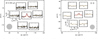 |
Fig. 1 Fine-structure line emission from µ Cephei, scaled in main-beam brightness temperatures (Rayleigh-Jeans equivalents), as seen in the individual upGreat pixels. Spectra are centered at the pixel positions (median spacings of 34″.4 and 15″.6 for the LFA and the HFA, respectively); Gaussian fits are overlaid in red and spectral baselines in orange. Gray-filled circles indicate the half-power beamwidths of 14″.1 and 6″.6 for the LFA and the HFA, respectively. Left : [OI] λ 63.2 μm emission (HFA, smoothed to 1.2 km s−1 channel spacing.). Right : [CII] λ 157.7 μm emission (LFA, polarization-averaged and smoothed to 9.6 km s−1 channel spacing, see Appendix B and Fig. B.1 for higher resolution). |
2.2 Far-infrared spectroscopy with SOFIA/EXES
The fine-structure lines of [FeII] (6D7/2 - 6D9/2) at λ25.9884 μm and of [SI] (3P1 - 3P2) at λ25.2490 μm were observed with the EXES spectrometer (Richter et al. 2018) in its high-medium mode (Fig. 2), offering a spectral resolving power of R = 50000 (approximately 6km s−1), with a slit width and length of 3″.23 and 31″.284, respectively. Half-power beamwidths amount to 3″.47 and 3″.41 for the [Fe II] λ 26.0 µm and [S I] λ 25.2 µm lines, respectively. The observations were carried out on SOFIA flight #288 (2016 March 16, project ID 04_0136, Harper et al. 2018), with on-target exposure times of 2688 s and 3456 s for the [Fe II] λ26.0 μm and [SI] λ25.2 μm lines, respectively, at 22° to 23° elevation. The chop-and-nod mode was used with beam separations of ±10″. The data were extracted and calibrated with the IDL-based Redux package (Clarke et al. 2015, version 1.0.2,), which contains instrument-specific developments based on Lacy et al. (2002). The processing steps included despiking, flatfielding, cleaning and undistorting (the latter step consists of the correction of the echelogram for optical distortions). The atmospheric transmission estimate was confirmed with a subsequent observation of Callisto in the same instrument setup (95% and 37% transmission for the [S I] λ 25.2 µm and the [Fe II] λ 26.0 µm lines, respectively). The measured flux, 2675 Jy in the [Fe II] λ 26.0 µm and [S I] λ 25.2 µm setups (after correcting for a 66% slit loss) agrees with the measurement of Forrest et al. (1980) of the satellite’s flux between λ16 µm and λ38 µm. The latter can be described, within errors, by a 155 K blackbody spectrum, yielding flux densities of 2715 Jy and 2660 Jy at the wavelengths of the [Fe II] λ 26.0 µm and [S I] λ 25.2 µm lines, respectively. Callisto’s angular diameter at the time of the EXES observations was 1″.50. We note that a scaling factor of 1.7 was applied after the slit-loss correction, so as to ensure consistency with the fluxes measured with the Long Wavelength Spectrometer (LWS) on the Infrared Space Observatory (ISO) (cf. EXES Handbook for Archive Users, Rev. 1.0, Fig. 12).
 |
Fig. 2 Fine-structure line emission in [O I] λ 63.2 µm (top left), [Fe II] λ 26.0 µm (top right), and [S I] λ 25.2 µm (bottom left, with the telluric H2O feature). Two-component Gaussian fits are overlaid as colored lines and all spectra normalized to unity at peak. Bottom right: zoom into the Gaussian fits (blue: [O I] λ 63.2 µm, red: [Fe II] λ 26.0 µm, green: [S I] λ 25.2 µm). |
Fine-structure line fluxes of µ Cephei.
2.3 Phenomenological description
The fine-structure emission lines of [C II] λ 157.7 µm and [O I] λ 63.2 µm are displayed in Fig. 1. Only the central pixels show significant emissions at the applied respective spectral resolutions, with signal-to-noise ratios of 6.7 and 6.5, respectively. The emissions from [Fe II] λ 26.0 µm and [S I] λ 25.2 µm have slightly different line profile shapes, as shown in Fig. 2. While the [O I] λ 63.2 µm line is generally broader, the [S I] λ 25.2 µm line shares with it the blueside wing. The red-side wings of the [Fe II] λ 26.0 µm and [S I] λ 25.2 µm lines almost agree and are less prominent than their counterpart in the [O I] λ 63.2 µm line. The low signal-to-noise ratio of the [C II] λ 157.7 µm line hinders a closer assessment of its profile. However, all four fine-structure line profiles studied here are single-peaked, in contrast to the CO emission with its double peaks at υLSR = 0 and 50kms−1 (De Beck et al. 2010). The [O I] λ 63.2 µm line fluxes measured by ISO-LWS are consistent within uncertainties of one to two σRMS (Table 1). Similar comparisons between secondary calibrators can be found in Appendix B. The radiative transfer analysis presented in the following accounts for the calibration uncertainties quoted in Table 1.
3 Excitation modeling
As mentioned in the introduction, the opacities involved in the atomic fine-structure line emissions require a radiative transfer model to constrain the physical and chemical conditions between the extended photosphere and the inner circumstellar envelope of µ Cephei. Because the densities and temperatures in the line-emitting regions are yet unconstrained, we allowed for excitations out of local thermodynamic equilibrium (LTE). Likewise, we considered the mixed transfer of line and continuum radiation (the latter comprises the contributions from the photospheric emission at the inner boundary and from dust grains toward the outer boundary). The ingredients of our non-LTE code are described in the following, while technical details can be found in Appendices E and F.
3.1 Physical model properties
3.1.1 Stellar parameters
The parameters of RSGs are notoriously controversial, which contributes to the RSG problem mentioned in the introduction. In many objects, including µ Cephei, this situation arises from the difficulty to separate brightness centroid shifts caused by photospheric activity from annual parallaxes, as demonstrated by Chiavassa et al. (2022, yet challenged by Kochanek 2023). Levesque et al. (2005, further references therein) assign the star to the Cepheus OB2-A association, for which they adopt a distance modulus (m – M)0 = 9.7, i.e., a distance of 870 pc. The asymmetry of the outer dust envelope of µ Cephei, as seen in the images of the Photodetector Array Camera and Spectrometer (PACS) on the Herschel Space Observatory (Maercker et al. 2022), suggests that it has been eroded by the UV radiation from the nearby OB association (as, e.g., in the case of NML Cygni, Schuster et al. 2006). However, this asymmetry is successfully explained by the motion of µ Cephei through its surrounding ISM and the resulting interaction (Maercker et al. 2022). We therefore surmise that the association of µ Cephei with Cep OB2-A is questionable. This doubt is further corroborated by combining various distance estimates. Here we used a distance of  pc, derived from a spectroscopically determined luminosity (Messineo et al. 2021) and a size measurement with infrared K-band interferometry (Perrin et al. 2005; Lacour 2010), which results in a photospheric radius of 762 R⊙ . More details can be found in Appendix G.
Several studies (Levesque et al. 2005; Shenoy et al. 2016; Montargès et al. 2019) infer photospheric temperatures at the higher end of the RSG range given by Farrell et al. (2020b). Here we adopted the mean temperature of RSGs of type M1, 3780 ± 62 K (Arentsen et al. 2019). While the uncertainty does not reflect the width of the underlying population, we note that it agrees with the spectroscopically derived temperatures reported for μ Cephei by Messineo et al. (2021), Teff = 3769 ± 74 K. We therefore adopted the MARCS model atmosphere (Gustafsson et al. 2008) used by Davies & Plez (2021), with Teff = 3800 K (MARCS stands for Model Atmospheres with a Radiative and Convective Scheme). In the non-rotating evolutionary tracks of Ekström et al. (2012), the resulting luminosity places the star at a total mass of 11 M⊙, with a main-sequence mass of 15 M⊙. While it is impossible to constrain the total mass of RSGs from the stellar luminosity and temperature alone (the resulting degeneracy, Farrell et al. 2020a, contributes to the RSG problem), we can infer the core mass during central He burning via the relationship
 (1)
(1)
(Farrell et al. 2020b), which yields Mcore ≃ 7 M⊙, leaving 4 M⊙ for the convective envelope. Another estimate of the stellar mass can be obtained from an empirical relation between surface gravity and luminosity (Messineo et al. 2021), which yields g =  g cm−2 and a median total mass of M* = 10 M⊙. The adopted stellar parameters are summarized in Table 2.
Main parameters for the early-M-type RSG model of µ Cephei.
3.1.2 Stellar wind model
The model follows the semi-empirical description of the wind of Betelgeuse, employed by Harper et al. (2001) to describe the spatial profile of the star’s radio emission, and adopted by Davies & Plez (2021) to study the impact of the wind on the optical and near-infrared spectrum. In the remainder of this paper, we refer to this description as early-M-type RSG model. Radiationhydrodynamic simulations (Freytag et al. 2024) suggest that the inner circumstellar envelope displays some clumpiness; for the outer envelope, the CO J = 2-1 maps (Northern Extended Millimeter Array, NOEMA, Montargès et al. 2019) provide direct evidence. The neutral, mixed atomic and molecular gas considered in our model is therefore unlikely to be the only gas phase. In Betelgeuse, a Te ~ 104 K hot plasma is required to generate the observed chromospheric lines (Harper et al. 2001). From a comparison with the radio flux, an area-filling factor of fA ≲ 0.25 has been inferred for the hot plasma. Without an approximate knowledge of the involved size scales, it is difficult to estimate the corresponding volume fraction of the ionized gas (and that of the atomic, neutral component as its complement). If one assumes an arbitrary number of spherical entities of a characteristic radius rn, immersed in a chromosphere confined between inner and outer radii ri and ro, respectively, it is straightforward to show that the ratio of their volume- and area-filling factors is given by  . Assuming
  for the cooler gas (i.e., the complement of the Betelgeuse value for the hot plasma), ri = 1.25 R* and ro = 1.85 R*2, and rn = (ro - ri)/2, we estimate
  . This is the average volume dilution for a power-law such as
  (where rc = 1.45 R* is the approximate distance of the chromosphere from the center of the star), which we adopt in the following (Fig. 3). However, later we indirectly account for the hot, partially ionized component by allowing for photo-chemistry triggered by the associated far-UV radiation.
 |
Fig. 3 Top: volume-filling factor of the cool clumps (black) and temperature profiles (red) of the early-M-type RSG models A (solid) and B (dashed). Center: densities of selected species from the FASTCHEM simulation, for model A. Bottom: same as the center but for model B. The color code for the displayed species is given in the bottom right corner. Solid lines refer to neutral and dashed lines to singly ionized species. For the definition of models A and B, see Section 4 and Fig. 4. |
Main characteristics of examined atomic fine-structure transitions.
3.2 Elemental and chemical abundances
A realistic description of the abundances of the atomic species considered here (C II, O I, S I, and Fe II) does not only require the knowledge of the elemental abundances at the stellar surface, but also a chemical model describing their uptake by the chemistry between the extended photosphere and inner circumstellar envelope. The elemental abundances of He, C, N and O are from the surface values of the SNAPSHOT models for the RSG phase (Farrell et al. 2020b, models C, D or E). Their model E has a stellar mass of 21.1 M⊙, and a photospheric temperature Teff = 3800 K corresponding to our photometric estimate given above (both stellar parameters are close to the upper limits in Montargès et al. 2019). The snapshot models were computed in an attempt to systematically relate the mass and composition of stellar cores to observable stellar surface properties. Ultimately, for fixed stellar model parameters (core mass and composition, convective envelope mass, and helium abundance profile), increasing the metallicity of the convective envelope increases the opacity and lowers the surface luminosity below the nuclear luminosity of that model, such that the star will reach equilibrium at a larger radius and lower Teff (Farrell et al. 2022). For Fe, we used as template the elemental abundance of Betelgeuse determined by the MAGIS project (Measuring Abundances of red super Giants with Infrared Spectroscopy, Taniguchi et al. 2025), and the abundances derived from it (Al, Ca, Cr, K, Mg, Na, Ni, Si, and Ti). In the absence of better information, all other elements were assumed to have a solar abundance (Asplund et al. 2009, further references therein). This mixture (summarized in Table A.1) reflects the uncertainties and the incompleteness of our knowledge of elemental abundances on the surfaces of RSG stars; a complete examination of the resulting bias remains to be done once more reliable values become available.
While a fully self-consistent chemical model is reserved for future work, we applied a thermal-equilibrium (TE) chemistry model, as an approximation motivated by the expected high densities. We used the FASTCHEM code (version 3, Stock et al. 2022) in its extension including the formation of condensates (Kitzmann et al. 2024). It predicts, for a given vertical gas temperature profile (as a function of gas pressure), the abundances of 523 neutral and charged gaseous species, and of 190 solid particles. Ionization fractions are inferred via the Saha equation, but photochemistry is not included (a caveat that will be discussed below).
3.3 Statistical equilibrium and radiative transfer
For the statistical-equilibrium calculations, we considered collisions with free electrons, H I, H2, and He. For the excitation of O I and C II by collisions with H2, we used separate rates for its ortho- and para spin-isomers, assuming thermal-equilibrium partitioning. Owing to the lack of rate coefficients for collisions of S I and Fe II with partners other than H I and free electrons, we applied scaling factors of (μX,H/μX,Y)1/2, where μ denotes the reduced mass of the colliding system, X stands for S I or Fe II, and Y for H2 or He. The same holds for collisions of C II with He. References to the available literature are summarized in Table 3.
The likelihood of deviations from LTE in an N-level system can be estimated by introducing a critical density ncrit above which a level i remains collisionally excited against spontaneous decay to level j,
 (2)
(2)
where Ai,j designates the Einstein coefficient of the transition, Nc = 4 is the number of the major colliding species (labeled with index k), n(k)/nH are their abundances with respect to the number of hydrogen nuclei, and  the collisional rate coefficients. The impact of non-LTE conditions on the line formation can then be assessed by the fraction of the emissivity that arises in regions where nH > ncrit. For most of the models and tracers discussed below, this fraction is close to unity. Unsurprisingly, for the two models retained below for closer analysis, the excitation temperature deviate from the gas temperatures by less than 3%, with the exception of the S I line in a high-temperature model (less than 9%).
For the [FeII] λ26.0 μm line, the collisional rate coefficients quoted in Table 3 are approximative for all partners except electrons (see Mendoza et al. 2023, for a summary). Those for collisions with H I (Yakovleva et al. 2019) do not contain transitions within the electronic ground-state quintuplet, and corresponding quantum-mechanical calculations are desirable. Accordingly, all hydrogen densities in our models are at least one to two orders of magnitude above the corresponding critical densities as defined by Equation (2). We therefore abstained from statistical equilibrium calculations for Fe II and assumed the population of its ground-state quintuplet to be in LTE.
For the other fine-structure lines, we only considered transitions within the electronic ground-state fine-structure triplets or doublets; the inclusion of all lines from a line list such as the Vienna Atomic Line Database (VALD3, Ryabchikova et al. 2015), would be prohibitive. The first electronically excited levels for C II, O I, and S I are at 61.87, 22.83, and 13.29 kK above ground, respectively. These levels can only be populated at the highest temperatures of our models through collisions in the wings of the involved Maxwellians. We corrected for them by scaling the levels populations of the ground-state triplets or doublets downward, assuming that LTE holds throughout the electronic excitations, using the partition functions of Barklem & Collet (2016). These corrections are moderate and amount to a factor close to unity, falling to 0.87 only for S I at 16 000 K. As a matter of fact, RSG spectra in the near-infrared Y and J bands contain no Fe II lines that would be useful for ionization balancing with the Saha equation, and only few lines from other ionized species (Taniguchi et al. 2025).
Our non-LTE radiative transfer code uses short characteristics to benefit from the simplifications facilitated by the spherical symmetry (see Appendix E for technical details). We considered the local trapping of spectral-line and continuum photons thanks to an escape-probability approach (Appendix F) and included the contribution of the stellar radiation at the inner boundary (approximated by a blackbody spectrum at Teff) to the excitation of the involved fine-structure levels. The convergence of the escape probability was accelerated by minimization of residua. The algorithm is computationally inexpensive; for O I, C II and S I, we therefore retained the non-LTE modeling for more accuracy, required to estimate the cooling effected by the [O I] and [C II] emissions (Appendix D).
3.4 Dust and gas opacities
3.4.1 Dust opacities
The spectral profiles of silicate absorption features in the ISM resemble those seen in the infrared spectrum of µ Cephei (Roche & Aitken 1984; Moneti et al. 2001). We therefore used the extinction curve of Draine & Lee (1984). Converting the visual extinction (Levesque et al. 2005 report AV = 2.01, de Wit et al. 2008 a source-intrinsic envelope contribution of 0.7) to column density (NH = AV · 2.21 × 1021 cm−2, Gϋver & Özel 2009) yields a mean hydrogen column of 6 × 1021 cm−2. Referring all line areas to that of the [O I] λ 63.2 µm line, the corrections of the resulting line ratios for the extinction in the foreground screen amount to at most 2.7%.
In the inner envelope, one must allow for the coexistence of atomic gas and dust. For the silicate dust, we refer again to the dielectric function from Draine & Lee (1984) with a Mathis et al. (1977) grain model, known as “astronomical silicates” and required for fitting the λ 10 µm dust feature. For an adequate reproduction of the [S I] λ 25.2 µm and [Fe II] λ 26.0 µm line area ratios, the addition of another dust species condensing at higher temperatures is required. For M-type (i.e., oxygen-rich) AGB stars, corundum (Al2O3) was identified by Höfner et al. (2016) as a promising candidate to explain the scattered-light observations and mid-infrared interferometry. We adopted it for the similarly oxygen-rich environment of µ Cephei and refer to Appendix A.2 for further details.
3.4.2 Gas opacities
As a refinement to the numerical solution of the mixed line and continuum radiative transfer, we included the opacities arising from the blend of ro-vibrational transitions and collision-induced absorptions due to all species predicted by the FASTCHEM TE model. The required opacity tables were generated by means of the OPTAB code (Hirose et al. 2022), assuming that all level populations are in LTE. The latter approximation is tolerable, given the weak contribution of these opacities (∆τ ≲ 0.03) to those of the continuum, which is the consequence of negligible pressure broadening.
3.5 Velocity field and line broadening
To closely describe the spectrally resolved line profiles, we tested various radial velocity prescriptions combining radiation-driven and ballistic (i.e., pressure-free) motions in the inner part of the envelope with a dust-driven wind in the outer parts. Ballistic motions starting at the stellar surface gravity of ≈0.5cm s−2 decelerate too fast to allow for a good description of the wings of the [O I] λ 63.2 µm line. The mechanisms driving winds in RSG stars are less well understood than those in their AGB equivalents (Gottlieb et al. 2022). A radiation-driven wind generally follows a so-called β-type velocity profile (Pauldrach et al. 1986), of the form
 (3)
(3)
which we adopted for the dust-accelerated part of the wind, with β = 0.5 and starting and final velocities of υr(rd) = 4km s−1 and υ∞ = 35km s−1 (De Beck et al. 2010), respectively. Since the observed atomic fine-structure lines mainly form within the dust condensation radius rd, they are not very sensitive to this component of the wind.
In the extended photosphere and chromosphere, the velocity field is more complex (Freytag et al. 2024). While substantial amounts of gas are levitated above the photosphere, a large fraction of this material falls back, creating “pseudo-convective” velocity patterns. Therefore, in a radially symmetric radiative transfer simulation of spatially unresolved observations, the assumed radial velocity profile is at best an instrument to reproduce the observed line shapes. In Appendix E.2, we show that the beam-averaged line profiles of optically thin emissions arising from upwelling and infalling gas cells (with some imbalance in spatial extent or brightness) can be equally well described by a centro-symmetric velocity field of the form
 (4)
(4)
with a photospheric levitation velocity υr(R*) = 16km s−1. The shape parameter α allows one to vary the profile between a linear one and a step function (for α << 1 and α >> 1, respectively); α ~ 1 provides a good fit to the observed line profile. Interestingly, these radial velocities compare to the differential velocities of Josselin & Plez (2007) derived from a correlation analysis of spectral masks applied to their visual spectra (ELODIE echelle spectrograph, Haute-Provence Observatory). The levitation velocity falls a factor of approximately four below the escape velocity at the stellar surface. Mass loss within the dust condensation radius therefore requires an acceleration mechanism. While the description of the radial velocity profile defined by Equations (3) and (4) is not unique, a more realistic picture is beyond the scope of this study.
Our spectra are not very sensitive either to the prescription of the line broadening. We assumed a constant macroturbulent component (e.g., Gray 2021) to which we added in quadrature a density-dependent component due to Alfvénic turbulence. Tessore et al. (2017) measured a photospheric magnetic field strength of B ≈ 1 Gauss (sightline component). With the Alfvén velocity  , where we set the effective density to the gas density because of the expected strong ion-neutral coupling (see Harper et al. 2022, section 6), a radiation-driven dense wind (ρ ~ 10−10g cm−3) becomes easily super-Alfvénic (υA ≈ 0.3 km s−1, implying an Alfvénic Mach number MA = υr(R*)/υA ~ 50). Further away, at 1.5 R* (the typical distance of the chromosphere from the center of the star) and beyond, the density falls to ρ ~ 10−14 g cm−3 and the conditions become sub-Alfvénic as long as the decrease of the magnetic field strength is not steeper than ∝r−1. At about 5 R*, the circular polarization of SiO masers may provide an estimate of B (Marinho et al. 2024), but for µ Cephei only upper limits are known so far. Under such conditions, the turbulent linewidth ∆υ(t) arising from undamped Alfvén waves scales as
  (Holzer et al. 1983). We therefore applied a prescription of the form
 (5)
(5)
with a macro-turbulent velocity dispersion  and a turbulence parameter κ(A) = 0.1. As an indication, for a typical early-M-type RSG model (see below), the velocity dispersions due to turbulence vary between 2.0 and 2.3 km s−1 at the photosphere and the outer model boundary (at 12.5 R⋆), respectively (in terms of 1/e full-widths: 5.66 and 6.51 km s−1, respectively). At all radii that are relevant to the line formation, this linebroadening component exceeds the thermal one, to which it is added in quadrature, by factors of 1.22 to 3.86 at the photosphere and the outer boundary, respectively.
3.6 Parameter study
To mitigate the impact of the distance uncertainty, for the initial analysis we used line-area ratios such as [O I]λ63/[O I]λ 145 and [O I]λ63/[CII]λ 158. As demonstrated by Watson (1985) for interstellar clouds and applied by Liu et al. (2001) to planetary nebulae, these ratios are well suited to constrain the density and temperature in the emitting region. In a similar approach to the analysis of fine-structure line emissions from RSGs, we modeled the excitation and line formation of these species on a grid of chromospheric densities and temperatures. For each grid point, we obtained the required abundance profiles from the corresponding TE chemistry model (two examples are shown in Fig. 3). To resolve ambiguities, we included the [O I]λ63/[S I]λ 25 and [O I]λ63/[Fe II]λ26 line-flux ratios in the analysis. As reference, we used the density and temperature profiles of the early-M-type RSG model of Harper et al. (2001, hereinafter referred to as standard model). Beyond the chromosphere, around a distance of 3 R⋆ from the center of the star, the density profile in the predominantly atomic gas phase can be described as a function of radius by a power law with index −2.74. In the same zone, the index for the temperature power law profile is around −0.9. We note that exponents of −1.33 and −0.80 would be expected for the adiabatic expansion of monatomic and molecular gas, respectively (cf. Montargès et al. 2019), but such a prescription ignores other contributions to cooling (e.g., spectral line cooling) and the local heating of the gas (e.g., gas-grain drag), which are discussed in Appendix D. For a parameter study, we linearly scaled the wind density with factors of log2 = −1.5 to 5.5 in steps of 0.5 (i.e., from 0.35 to 45.25), and add log-normal temperature profiles to that of the standard model, of width 0.86 R⋆ and centered at the chromosphere. Such a prescription allows for a pronounced yet smooth temperature variation across the chromosphere. The amplitudes of this additional component range from 0% to 56% of the chromospheric temperature of the standard model, in steps of 4%. The results obtained on this 15 × 15 grid are schematically shown in Fig. 4; temperatures and densities refer to the chromospheric temperature maximum.
 |
Fig. 4 Fine-structure line excitation analysis on a gas densitytemperature grid of early-M-type RSG models, including photochemical enhancement of the [C II]λ158 line flux by a factor 10. Densities and temperatures refer to the location of the chromospheric temperature maximum; blue lines indicate iso-density contours. The colored areas delimit the (ng, Tg) loci where the model-predicted line-area ratios agree with the observed ones within ±1.2σrms: [OI]λ63/[OI]λ145 (Gray), [OI]λ63/[CII]λ158 (cyan), [O I]λ63/[S I]λ25 (red), and [O I]λ63/[Fe II]λ26 (green). The solutions in the red-filled area are compatible with all four measured flux ratios with a 60% likelihood (model A). If the [O I]λ63/[S I]λ25 ratio is omitted, a second solution emerges (model B). The locations of the corresponding least-square solutions are labeled with black dots. The orange abscissa on the top indicates the volume-averaged magnetic field strengths required for virial equilibrium. For details see text. |
4 Results
The most striking result of the parameter study is the impossibility to reproduce the observed [O I]λ63/[C II]λ158 ratio. For the standard model, with its chromospheric peak temperature of 3700 K (as in Harper et al. 2001), this ratio exceeds the observed one by two orders of magnitude. For a model with a 5215 K hot chromosphere, and a factor four denser wind, the discrepancy is reduced to an order of magnitude. In other words, enhancing the modeled [C II] λ 157.7 µm line area by a factor 10 yields a fully concordant solution. While applying such a scaling may seem arbitrary, we demonstrate below that this can be achieved with the photo-chemistry of the available reservoirs of C I and CO. We refer to this solution as model A.
Because virtually all level populations encountered in these excitation models are close to LTE, the dependence of the line area ratios on the gas density is an indirect one. For lower densities, the optical depths decrease, which gives a higher weight to the contributions from warmer regions and thus higher emissivities. The O I line ratio is not very sensitive to the temperatures either, which is readily understood by comparing the level energies in the 3P ground state triplet (228 and 327 K above ground) with the encountered gas temperatures ranging from 3700 to 5700 K. The fairly low significance of the [O I]λ 145 and [C II]λ 158 detections, with signal-to-noise ratios of 3–5, introduces a further complication. The density and temperature of the chromosphere are therefore only loosely constrained. The inclusion of the [OI]λ 63/[SI]λ 25 and [OI]λ 63/[FeII]λ 26 line ratios helps overcome this limitation. Although the latter ratio exhibits an ambiguity (the same flux ratio can apply to two distinct density scaling factors), in combination with the other line ratios the best-matching result is concordant. If one removes the constraint imposed by the [O I]λ 63/[S I]λ 25 ratio (keeping the factor 10 scaling of the modeled [C II]λ 158 line area), a second solution emerges, that is denser than the standard model by a factor 23, but less hot, with a chromospheric temperature of 4375 K (model B). This approach can be rationalized with the fact that in oxygen-rich AGB stars, sulfur chemistry tends to be out of equilibrium (Agúndez et al. 2020), which would invalidate our TE chemistry approach for this element. Alternatively, the [O I]λ 63/[S I]λ 25 line ratio can be recovered by removing the excess of S I through its photo-ionization. Comparing the ionization potentials of C II and S I (Table 3), this appears to be a natural consequence of carbon photochemistry. The origin of the required UV excess will be discussed further in the next section. As shown in Appendix C, the factor 10 scaling of the modeled [C II]λ 158 line area in the above parameter study can be replaced by correcting the TE-abundances for photochemistry. The resulting line areas matching the observations for both models A and B are summarized in Table 4. We note in passing that without the addition of alumina, condensing at higher temperatures than silicates, the fluxes of the [S I] λ 25.2 µm and [FeII] λ 26.0 µm lines are over-predicted by 11% to 14% in model A, and by 86% to 105% in model B.
The continuum fluxes of models A and B (Table C.1) are not too far from the observed radio (free-free) and far-infrared fluxes. The main carrier of the radio opacity are free-free transitions of H−, followed by those of He−. We computed the free-free flux following Harper et al. (2001, their Eqs. (5) and (6)), with H I, He I, and e− densities from the FASTCHEM TE chemistry, assuming that the radio flux is emitted from the same gas phase as the fine-structure lines. Within the uncertainties derived from a visibility fit to archival 8.14 GHz VLA data, model A leaves space for a radio flux contribution from the UV-emitting hot gas phase driving the photo-chemistry, which is difficult to evaluate, also in view of a potential variability of the radio flux. Model A also provides a better match for the far-infrared continuum fluxes. While their attenuation by the cooler circumstellar envelope at more than 40 au from the stellar surface is taken into account, the dust emission of this foreground is not reflected by our model focusing on the fine-structure line emissions.
Both models provide a good fit to the [O I]λ 63 line profile and flux, as shown in Fig. 5. Replacing the stellar wind by an inflow would allow for a still acceptable fit. This reflects the fact that with our data, we cannot easily decide which fraction of the stellar wind escapes, and which one falls back to the star. We note, though, that the second maximum of our SiO density profile (Fig. 6) matches, at the adopted distance, the extent of the SiO (v = 1,J = 1–0) masers (VLBI, Colomer 1993). The radial velocities encountered in this zone reproduce the end velocities of Marinho et al. (2024). The density and radial velocity profiles adopted by our modeling entail that the massloss rate cannot be constant in time, reminiscent of scenarios involving superwind phases of enhanced mass loss (Decin et al. 2006). The mass loss rate at the outer boundary of our model is only weakly constrained and amounts to 0.5 × 10⁻⁶ M⊙ yr−1 if one accounts for the (quantitatively uncertain) volume dilution of the cool gas. Adjusting the mass-loss rates obtained from fitting CO line profiles (De Beck et al. 2010, for d = 390 pc, yet a flawed systemic velocity) and dust spectral energy distributions (Shenoy et al. 2016, d = 870 pc) to our distance (421 pc) yields 2.3× 10⁻⁶ M⊙ yr−1 and 0.9×10⁻⁶ M⊙ yr−1, respectively, while the mass loss from the CO J = 2–1 interferometry of Montargès et al. (2019, d = 641 pc) yields 1.1 × 10⁻⁶M⊙ yr−1.
We also note that our models reproduce the shape and sightline-velocity of the H I λ 21 cm line profile measured by Gérard et al. (2024). The authors speculate that the blue-shifted part of a potential double-peak H I profile blends with Galactic emissions, difficult to avoid in single-dish observations. Our models suggest that this is not the case, and predicts line fluxes at ~60% of the observed value (Table 4). This leaves space for an H I reservoir outside the outer model boundary, but originating from the star.
Line fluxes for the early-M-type RSG models A and B after corrections for photochemistry (absolute values; ratios with respect to observed fluxes in brackets).
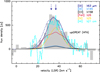 |
Fig. 5 Model spectra of the [O I] λ 63.2 µm line (solid dark blue line for a wind and dashed for inflow) and the [O I] λ 145.5 µm line (light blue), for d = 421 pc and a systemic velocity of υLSR = 36.0 km s−1. The observed λ 63.2 µm spectrum is shown as a gray-filled histogram underneath. Blue arrows mark the systemic velocities discussed in the main text (solid arrow: our model, υLSR = 36kms−1; dashed arrow: υLSR = 32.7 kms−1, Montargès et al. 2021). Model spectra for [CII] λ 157.7 μm, [FeII] λ 26.0 µm, and [S I] λ 25.2 µm are overlaid in black, red, and yellow, respectively. The H I λ 21 cm spectrum (cyan) is scaled, for better visibility. |
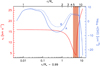 |
Fig. 6 Profiles of radial velocity (red) and of SiO density (the solid blue line is for model A and dashed blue one is for model B). The dark-salmon filled area indicates the velocity range compatible with the range of sightline velocities of SiO (v = 1, J = 2–1) maser components (υLSR = 19 to 43km s−1, Marinho et al. 2024) for a systemic velocity of 36.0 km s−1 (obtained through profile fitting of the [O I]λ63 line). The dotted blue line displays the largest projected distance of v = 1, J = 1–0 SiO maser spots from the star (Colomer 1993, for 421 pc distance). |
5 Discussion
As shown in Fig. 7, the predominant contribution to the observed fine-structure line fluxes originates in the chromosphere. The far-UV flux required for driving the carbon photochemistry most likely arises from energy dissipation in shocks, which also explains the chromospheric emission lines. As shown by radiation-hydrodynamic (RHD) simulations (Freytag et al. 2024), these shocks form in response to the stellar pulsation and the encounters between the wind and substantial inward motions. Although their RHD models are for stars of up to 8 M⊙, there is a priori no reason to rule out shock formation in the atmospheres of red supergiants. As a matter of fact, the infall velocities of the gas above the shock may be substantial, and we re-emphasize that the adopted distribution of radial velocities matching the observed [O I] λ 63.2 µm line profile does not rule out inward motions. As stated by Freytag et al. (2024), a more quantitative description of these shocks requires a higher numerical resolution, combined with non-LTE radiative transfer.
We note that the ratio of the radius to the mass of our stellar model, 69.3 R⊙/M⊙, is close to that of the 8 M⊙ model of Freytag et al. (2024, 75.3 R⊙/M⊙). For a given temperature and chemical composition, this ratio scales with that of pressure scale height to stellar radius, Hp/R⋆. In mixing length theory, the characteristic length scale over which a given convection element dissipates is generally obtained from scaling Hp (e.g., Kippenhahn et al. 2012) with a parameter calibrated against observations or RHD simulations (e.g., Goldberg et al. 2022). The cross-sectional width of a convection element can then be estimated by mass conservation (Stein & Nordlund 1998), which requires that the upward mass flux equals that through the upper boundary of the convection cell (neglecting the stellar wind). In summary, for given temperature, density and chemical composition, the number of convection cells scales coarsely with (R*/M*)−2. While the analogy should not be taken too far, two causes of great dimming events work in AGB stars and RSGs alike (namely, Rayleigh-Taylor plumes and convective downdraft with subsequent rebound, both creating quickly cooling, overshooting material, Freytag et al. 2024).
Observationally, the RHD models are not only backed by shock tracers. The underlying vigorous motions in the extended stellar atmosphere are directly evidenced by near-infrared interferometric spectroscopy of ro-vibrational CO emissions (Ohnaka et al. 2017), and indirectly by means of optical spectro-polarimetry. As demonstrated by López Ariste et al. (2023), the observed Stokes Q and U line profiles of µ Cephei are due to the depolarization of the underlying continuum and allow one to infer the height of plumes forming in the Rayleigh-Taylor instabilities that build up in the upflowing gas. They extend to up to 1.3 R⋆, which is close to the location of the chromosphere in our model.
It is interesting to note that without invoking shocks, photochemistry is expected to arise in the outer envelope, where the molecular gas is exposed to the interstellar radiation field (ISRF), i.e., beyond the CO clumps resolved by NOEMA observations (Montargès et al. 2019). Conversely, the [C II] λ 157.7 µm line emission originates from the chromosphere, and not the circumstellar envelope: we re-emphasize that the line is not detected in the annular average of the off-center pixels of upGREAT, at 31″ offset. A similar situation is observed in the prototypical carbon star IRC+10216 (Reach et al. 2022; Jeste et al. 2023). It is not excluded that photons from the ISRF capable of ionizing carbon travel through a patchy circumstellar envelope, as also proposed by Agúndez et al. (2010) to explain the presence of warm water vapor around IRC+10216 (Decin et al. 2010).
In Betelgeuse, the putative companion mentioned in the introduction could also produce UV emissions through mass transfer. The detection of tracers of photo-chemistry in the AGB-main sequence binary W Aql (Danilovich et al. 2024) lends further support to this hypothesis. However, if similar mechanisms were dominating in Betelgeuse, they would mask the observed correlation of the λ 300 nm continuum flux with the stellar pulsation (Dupree et al. 1987, 1990, with a ∼400 d period), while the companion orbits with a ∼2000 d period (Dupree et al. 2026). Extrapolating to µ Cephei, without further observations we view the possibility of mass-transfer induced photochemistry with some degree of reservation.
Another potentially important mechanism involves cosmic-ray generated UV radiation. The rates of the cosmic-ray induced ionization of H I and H2, ζH2, is uncertain. For ζH2 = 10−16 s−1, Heays et al. (2017, further references therein) deduce the ionization rate of carbon, χc = 2.60 × 10⁻¹⁴ s−1. In our model, close to the photosphere, most hydrogen nuclei are in the form of H I, and the appropriate primary ionization rate per hydrogen atom would be ζH I = 1.78 × 10⁻¹⁶ (Indriolo et al. 2015, for the diffuse, partially atomic ISM). In equilibrium with the recombination of C II, occurring at a rate
 (6)
(6)
(UMIST Database for Astrochemistry 2022, Millar et al. 2024), i.e., balancing the photo-ionization and recombination of atomic carbon ( ), we obtain the expression
![Mathematical equation: n_\mathrm{\ion{C}{ii}} \approx \left(0.01\,n_\mathrm{\ion{C}{i}}[\mathrm{cm^{-3}}]\left(\frac{T}{300\,\mathrm{K}}\right)^{0.29}\exp{\left(\frac{17.60\,\mathrm{K}}{T}\right)}\right)^{1/2}\mathrm{cm^{-3}}](/articles/aa/full_html/2026/07/aa60113-26/aa60113-26-eq20.png) (7)
(7)
where we assumed that the free electrons are predominantly provided by the ionization of C I (i.e., ne- ≈ nC II). Up to 0.14 and 0.19 stellar radii above the photosphere, for models A and B, respectively, cosmic-ray generated UV radiation can produce orders of magnitude more C II than deduced from the TE chemistry (through the Saha equation). In the chromosphere (i.e., at approximately 0.5 stellar radii above the photosphere, close to the peak of the [C II]λ 158 contribution function, Fig. 7), this C II yield falls three orders of magnitude below that of the TE chemistry. This leaves shock-generated UV radiation as a more promising explanation for the observed C II over-abundance in the chromosphere. In view of the uncertainties of these estimates, such a conclusion should be taken with a pinch of salt and more detailed models are reserved for future work.
Last, but not least, we do not rule out the possibility that we underestimate the carbon abundance. Singh et al. (2023) find variations of the 12C/13C ratio in the molecular envelope of VY CMa which they trace back to non-classical dredge-up of nucleosynthesis products (for an overview see Ziurys & Richards 2025). The mixing mechanism leading to a substantial over-abundance of carbon on the stellar surface remains to be identified, though. In RSGs, mixing through rotation is less efficient than by convection (Heger & Langer 2000), but the surface composition of models including rotation on the main sequence changes much faster than that of non-rotating models (Ekström et al. 2012). Actually, in the former models, more carbon is processed into nitrogen. This is consistently predicted by the Heger & Langer (2000) and Ekström et al. (2012) models (C/O ≈ 0.2 by number), while the C/O ratio of the non-rotating models is higher by a factor of about two. If the required order-of-magnitude increase of the C II abundance over that of TE chemistry was solely due to a higher elemental surface abundance of carbon, it would push the C/O ratio to ∼3, which is at odds with the stellar evolution models. An increased oxygen abundance leaving the C/O ratio unchanged would lead to an under-prediction of the observed [O I]λ 63 flux, owing to the increased optical depth. Resolving this issue by suggesting an exposure of the CNO layer due to intense mass ejections would require a close examination of the historic record.
In summary, these results corroborate the complex dynamics in the chromosphere, making a pressure equilibrium between the gravitational, magnetic, thermal and turbulent components highly unlikely. It is nevertheless instructive to estimate the magnetic field strength (the only quantity missing in the model description) using the generalized virial theorem (Chandrasekhar & Fermi 1953), averaging its terms over a time interval ∆t long enough to ensure equilibrium3, i.e.,
 (8)
(8)
yet short compared to the stellar evolution timescale. For a spherical shell confined between inner and outer radii ri and ro, respectively, the kinetic and thermal energies K and Θ, respectively, are given by
 (9)
(9)
(where the pressure p includes a contribution from the adopted turbulence), and the magnetic energy M and potential energy Ω (neglecting the self-gravitation of the chromosphere) by
 (10)
(10)
The surface term S is negligible in most applications of the virial theorem; here we must keep it because it does not vanish on the surface of the modeled region (bounded by the photosphere and the inner circumstellar envelope):
 (11)
(11)
For a constant magnetic field, the resulting field strengths amount to approximately 1.6 G and 0.7 G for models A and B, respectively. For a dipole field (B ∝ r−3), the values at the stellar surface amount to 1.3 G and 0.6 G. They are close to the photospheric value of ≈1 G (Tessore et al. 2017) and fall below the upper limit derived from SiO maser polarization (Marinho et al. 2024). The wind is then sub-Alfvénic beyond 1.12 R⋆, i.e., in the extended photosphere and in the chromosphere, which is a prerequisite for our description of turbulence.
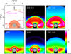 |
Fig. 7 Top left: meridional cuts of line-profile-averaged total optical depths into the envelope (τlos = 0.7 contours where emissions from the inside are attenuated by more than 50%), for model B, with [O I] λ 63.2 µm (dark red), [OI] λ 145.5 µm (bright red), [C II] λ 157.7 µm (black), [FeII] λ 26.0 µm (magenta), and [S I] λ 25.2 µm (gold). Spectral-line opacities dominate the [O I]λ145, [O I]λ63 and [C II]λ 158 transitions, while in [FeII]λ 26 and [S I]λ 25, the λ25 µm continuum opacity prevails. The gray disk represents the extent of the stellar photosphere, the salmon-filled area that of the chromosphere. The sightline to the observer is indicated by the black arrow. Top center to bottom right: contribution functions (i.e., the integrands of Eq. (E.1), normalized to unity at peak) for the respective emissions. |
6 Conclusions
Infrared fine-structure lines are useful tracers of physical and chemical conditions in the immediate vicinity of red supergiants, as they do not suffer from strong self-absorption or dust extinction in circumstellar and interstellar foregrounds. In combination with chemical models, they provide a supplementary tool to further constrain stellar surface abundances, which are hitherto fraught with uncertainties. The largest contributions to the far-infrared line fluxes of C ii, O I, S I, and Fe II studied in this work come from the chromosphere. We applied a dedicated radiative transfer code, backed by chemical thermal-equilibrium models, to identify two solutions for the density and temperature layering which agree with the measured line fluxes within the observational uncertainties. At the chromospheric temperature maximum, their gas pressures coincide within a factor of four. However, matching the observed [C II]λ 158 and, to a lesser degree, [S I]λ 25 line fluxes requires a substantial contribution from photo-chemistry, while the [Fe II]λ 26 flux can also be adjusted by small corrections of the elemental abundance. To move toward improved stellar surface abundances, the source of the far-UV radiation driving the photo-chemistry – most likely shocks forming in encounters of the stellar wind with an inflow of gas, and, potentially, cosmic ray impacts in the extended photosphere – must be fully characterized. Our spatially unresolved observations do not provide an unequivocal description of the gas kinematics and turbulence near the star. Nevertheless, the high spectral resolutions achieved in this work and our modeling enable us to estimate the characteristic chromospheric velocities and heights in agreement with other studies. In particular, the H I λ 21 cm line emission, and the location and velocities of the SiO masers are reproduced by the two models.
Data availability
All tables and reduced spectra are available at the CDS via https://cdsarc.cds.unistra.fr/viz-bin/cat/J/A+A/711/A305
Acknowledgements
We dedicate this work to the memories of Karl M. Menten and Göran Sandell. We thank the SOFIA observatory staff and instrument teams for their dedication to the execution of these observations, and the referee, Guillermo Quintana-Lacaci, for an insightful and careful review of the manuscript. GREAT was a development by the MPI für Radioastronomie and the KOSMA/Universität zu Köln, in cooperation with the DLR Institut für Optische Sensorsysteme. The instrument development was financed by the participating institutes, by the German Aerospace Center (DLR) under Grants 50 OK 1102, 1103, and 1104, and within the Collaborative Research Centre 956, funded by the Deutsche Forschungsgemeinschaft (DFG). SOFIA was jointly operated by the Universities Space Research Association, Inc. (USRA), under NASA Contract No. NAS2-97001, and the Deutsches SOFIA Institut (DSI) under DLR Contracts No. 50 OK 0901 and No. 50 OK 1301 to the University of Stuttgart. This work was supported by the Action Thématique Physique Stellaire of CNRS/INSU PN ASTRO co-funded by CEA and CNES. G.M.H. acknowledges support provided by NASA SOFIA Cycle 4 grant SOF 04-0136 issued by USRA. H.W. enjoyed discussions with Lynn D. Matthews and Keiichi Ohnaka, and thanks the Laboratoire d’astrophysique de Bordeaux for hospitality.
References
- Agúndez, M., Cernicharo, J., & Guélin, M. 2010, ApJ, 724, L133 [CrossRef] [Google Scholar]
- Agúndez, M., Martínez, J. I., de Andres, P. L., Cernicharo, J., & Martín-Gago, J. A. 2020, A&A, 637, A59 [Google Scholar]
- Al-Shaqsi, N., Horchani, R., Ikot, A. N., Okorie, U. S., & Jelassi, H. 2025, Eur. Phys. J. Plus, 140, 696 [Google Scholar]
- Anderson, J. P., Dessart, L., Gutiérrez, C. P., et al. 2018, Nat. Astron., 2, 574 [NASA ADS] [CrossRef] [Google Scholar]
- Arentsen, A., Prugniel, P., Gonneau, A., et al. 2019, A&A, 627, A138 [NASA ADS] [CrossRef] [EDP Sciences] [Google Scholar]
- Asplund, M., Grevesse, N., Sauval, A. J., & Scott, P. 2009, ARA&A, 47, 481 [CrossRef] [Google Scholar]
- Bahcall, J. N., & Wolf, R. A. 1968, ApJ, 152, 701 [Google Scholar]
- Barinovs, Ǧ., van Hemert, M. C., Krems, R., & Dalgarno, A. 2005, ApJ, 620, 537 [NASA ADS] [CrossRef] [Google Scholar]
- Barklem, P. S., & Collet, R. 2016, A&A, 588, A96 [NASA ADS] [CrossRef] [EDP Sciences] [Google Scholar]
- Barlow, M. J. 1999, in IAU Symposium, 191, Asymptotic Giant Branch Stars, eds. T. Le Bertre, A. Lebre, & C. Waelkens, 353 [Google Scholar]
- Baudry, A., Wong, K. T., Etoka, S., et al. 2023, A&A, 674, A125 [NASA ADS] [CrossRef] [EDP Sciences] [Google Scholar]
- Begemann, B., Dorschner, J., Henning, T., et al. 1997, ApJ, 476, 199 [NASA ADS] [CrossRef] [Google Scholar]
- Bell, K. L., Berrington, K. A., & Thomas, M. R. J. 1998, MNRAS, 293, L83 [CrossRef] [Google Scholar]
- Bernat, A. P. 1977, ApJ, 213, 756 [Google Scholar]
- Biermann, L. 1951, Z. Astrophys., 29, 274 [NASA ADS] [Google Scholar]
- Blakely, D., Johnstone, D., Stolker, T., et al. 2025, AJ, 169, 152 [Google Scholar]
- Boboltz, D. A., & Marvel, K. B. 2000, ApJ, 545, L149 [Google Scholar]
- Boesgaard, A. M., & Boesgaard, H. 1976, ApJ, 205, 448 [NASA ADS] [CrossRef] [Google Scholar]
- Bohren, C. F., & Huffman, D. R. 1983, Absorption and scattering of light by small particles (John Wiley & Sons) [Google Scholar]
- Brown, J. M., Evenson, K. M., & Zink, L. R. 1994, ApJ, 431, L147 [Google Scholar]
- Chandrasekhar, S., & Fermi, E. 1953, ApJ, 118, 116 [Google Scholar]
- Chiavassa, A., Kudritzki, R., Davies, B., Freytag, B., & de Mink, S. E. 2022, A&A, 661, L1 [NASA ADS] [CrossRef] [EDP Sciences] [Google Scholar]
- Civiš, S., Kramida, A., Zanozina, E. M., et al. 2024, ApJS, 274, 32 [Google Scholar]
- Clarke, M., Vacca, W. D., & Shuping, R. Y. 2015, in Astronomical Society of the Pacific Conference Series, 495, Astronomical Data Analysis Software an Systems XXIV (ADASS XXIV), eds. A. R. Taylor, & E. Rosolowsky, 355 [Google Scholar]
- Clegg, P. E., Ade, P. A. R., Armand, C., et al. 1996, A&A, 315, L38 [NASA ADS] [Google Scholar]
- Colomer, F. 1993, in Astrophysical Masers, 412, eds. A. W. Clegg, & G. E. Nedoluha, 429 [Google Scholar]
- Colomer, F., Graham, D. A., Krichbaum, T. P., et al. 1992, A&A, 254, L17 [NASA ADS] [Google Scholar]
- Cooksy, A. L., Blake, G. A., & Saykally, R. J. 1986, ApJ, 305, L89 [NASA ADS] [CrossRef] [Google Scholar]
- Courant, R. 1988, Differential and Integral Calculus (John Wiley & Sons, Ltd), 315 [Google Scholar]
- Crosas, M., & Menten, K. M. 1997, ApJ, 483, 913 [NASA ADS] [CrossRef] [Google Scholar]
- Danilovich, T., Malfait, J., Van de Sande, M., et al. 2024, Nat. Astron., 8, 308 [CrossRef] [Google Scholar]
- Davies, B., & Beasor, E. R. 2018, MNRAS, 474, 2116 [NASA ADS] [CrossRef] [Google Scholar]
- Davies, B., & Beasor, E. R. 2020a, MNRAS, 496, L142 [NASA ADS] [CrossRef] [Google Scholar]
- Davies, B., & Beasor, E. R. 2020b, MNRAS, 493, 468 [NASA ADS] [CrossRef] [Google Scholar]
- Davies, B., & Plez, B. 2021, MNRAS, 508, 5757 [NASA ADS] [CrossRef] [Google Scholar]
- De Beck, E., Decin, L., de Koter, A., et al. 2010, A&A, 523, A18 [NASA ADS] [CrossRef] [EDP Sciences] [Google Scholar]
- de Natale, P., Bellini, M., Goetz, W., Prevedelli, M., & Inguscio, M. 1993, Phys. Rev. A, 48, 3757 [Google Scholar]
- de Wit, W. J., Oudmaijer, R. D., Fujiyoshi, T., et al. 2008, ApJ, 685, L75 [NASA ADS] [CrossRef] [Google Scholar]
- de Zeeuw, P. T., Hoogerwerf, R., de Bruijne, J. H. J., Brown, A. G. A., & Blaauw, A. 1999, AJ, 117, 354 [Google Scholar]
- Decin, L. 2021, ARA&A, 29, 274 [Google Scholar]
- Decin, L., Hony, S., de Koter, A., et al. 2006, A&A, 456, 549 [NASA ADS] [CrossRef] [EDP Sciences] [Google Scholar]
- Decin, L., Agúndez, M., Barlow, M. J., et al. 2010, Nature, 467, 64 [NASA ADS] [CrossRef] [Google Scholar]
- Deutsch, L. 1956, ApJ, 123, 210 [Google Scholar]
- Draine, B. T. 2011, Physics of the Interstellar and Intergalactic Medium (Princeton University Press) [Google Scholar]
- Draine, B. T., & Lee, H. M. 1984, ApJ, 285, 89 [NASA ADS] [CrossRef] [Google Scholar]
- Dupree, A. K., & Montargès, M. 2025, Galaxies, 13, 50 [Google Scholar]
- Dupree, A. K., Baliunas, S. L., Guinan, E. F., et al. 1987, ApJ, 317, L85 [Google Scholar]
- Dupree, A. K., Baliunas, S. L., Guinan, E. F., Hartmann, L., & Sonneborn, G. 1990, in Astronomical Society of the Pacific Conference Series, 11, Confrontation Between Stellar Pulsation and Evolution, eds. C. Cacciari & G. Clementini, 468 [Google Scholar]
- Dupree, A. K., Cristofari, P. I., MacLeod, M., & Kravchenko, K. 2026, ApJ, 998, 50 [Google Scholar]
- Eckes, M., Gibert, B., De Sousa Meneses, D., Malki, M., & Echegut, P. 2013, Phys. Chem. Miner., 40, 287 [Google Scholar]
- Ekström, S., Georgy, C., Eggenberger, P., et al. 2012, A&A, 537, A146 [Google Scholar]
- Farrell, E. J., Groh, J. H., Meynet, G., & Eldridge, J. J. 2020a, MNRAS, 494, L53 [NASA ADS] [CrossRef] [Google Scholar]
- Farrell, E. J., Groh, J. H., Meynet, G., et al. 2020b, MNRAS, 495, 4659 [NASA ADS] [CrossRef] [Google Scholar]
- Farrell, E., Groh, J. H., Meynet, G., & Eldridge, J. J. 2022, MNRAS, 512, 4116 [NASA ADS] [CrossRef] [Google Scholar]
- Forrest, W. J., Houck, J. R., & McCarthy, J. F. 1980, Icarus, 41, 340 [Google Scholar]
- Freytag, B., Höfner, S., Aringer, B., & Chiavassa, A. 2024, A&A, 692, A223 [NASA ADS] [CrossRef] [EDP Sciences] [Google Scholar]
- Froese Fischer, C., & Saha, H. P. 1983, Phys. Rev. A, 28, 3169 [Google Scholar]
- Froese Fischer, C., & Tachiev, G. 2004, Atomic Data Nucl Data Tables, 87, 1 [Google Scholar]
- Gaia Collaboration (Brown, A. G. A., et al.) 2021, A&A, 649, A1 [NASA ADS] [CrossRef] [EDP Sciences] [Google Scholar]
- Gaia Collaboration (Vallenari, A., et al.) 2023, A&A, 674, A1 [NASA ADS] [CrossRef] [EDP Sciences] [Google Scholar]
- Gérard, E., van Driel, W., Matthews, L. D., et al. 2024, A&A, 692, A54 [NASA ADS] [CrossRef] [EDP Sciences] [Google Scholar]
- Gérard, E., van Driel, W., Matthews, L. D., et al. 2025, A&A, 704, A186 [NASA ADS] [CrossRef] [EDP Sciences] [Google Scholar]
- Gilliland, R. L., & Dupree, A. K. 1996, ApJ, 463, L29 [Google Scholar]
- Gilman, R. C. 1974, ApJS, 28, 397 [NASA ADS] [CrossRef] [Google Scholar]
- Goldberg, J. A., Jiang, Y.-F., & Bildsten, L. 2022, ApJ, 929, 156 [NASA ADS] [CrossRef] [Google Scholar]
- Goldreich, P., & Scoville, N. 1976, ApJ, 205, 144 [NASA ADS] [CrossRef] [Google Scholar]
- Gottlieb, C. A., Decin, L., Richards, A. M. S., et al. 2022, A&A, 660, A94 [CrossRef] [EDP Sciences] [Google Scholar]
- Gray, D. F. 2021, The Observation and Analysis of Stellar Photospheres, 4th edn. (Cambridge University Press) [Google Scholar]
- Gry, C., Swinyard, B., Harwood, A., et al. 2003, The ISO Handbook, Volume III – LWS – The Long Wavelength Spectrometer [Google Scholar]
- Guan, X., Stutzki, J., Graf, U. U., et al. 2012, A&A, 542, L4 [NASA ADS] [CrossRef] [EDP Sciences] [Google Scholar]
- Guinan, E., Wasatonic, R., Calderwood, T., & Carona, D. 2020, Astronomer’s Telegram, 13512, 1 [Google Scholar]
- Gustafsson, B., Edvardsson, B., Eriksson, K., et al. 2008, A&A, 486, 951 [NASA ADS] [CrossRef] [EDP Sciences] [Google Scholar]
- Güver, T., & Özel, F. 2009, MNRAS, 400, 2050 [Google Scholar]
- Haas, M. R., Hollenbach, D., & Erickson, E. F. 1991, ApJ, 374, 555 [Google Scholar]
- Haas, M. R., Glassgold, A. E., & Tielens, A. G. G. M. 1995, in Astronomical Society of the Pacific Conference Series, 73, From Gas to Stars to Dust, eds. M. R. Haas, J. A. Davidson, & E. F. Erickson, 397 [Google Scholar]
- Haris, K., & Kramida, A. 2017, ApJS, 233, 16 [Google Scholar]
- Harper, G. M., Brown, A., & Lim, J. 2001, ApJ, 551, 1073 [NASA ADS] [CrossRef] [Google Scholar]
- Harper, G. M., Richter, M. J., Ryde, N., et al. 2009, ApJ, 701, 1464 [Google Scholar]
- Harper, G. M., Brown, A., Guinan, E. F., et al. 2017, AJ, 154, 11 [Google Scholar]
- Harper, G. M., DeWitt, C. N., Richter, M., et al. 2018, in American Astronomical Society Meeting Abstracts, 232, 325.01 [Google Scholar]
- Harper, G. M., DeWitt, C. N., Richter, M. J., et al. 2020a, ApJ, 893, L23 [NASA ADS] [CrossRef] [Google Scholar]
- Harper, G. M., Guinan, E. F., Wasatonic, R., & Ryde, N. 2020b, ApJ, 905, 34 [Google Scholar]
- Harper, G. M., Chambers, E., Vacca, W. D., et al. 2021, AJ, 162, 246 [Google Scholar]
- Harper, G. M., Ayres, T. R., & O’Gorman, E. 2022, ApJ, 932, 57 [NASA ADS] [CrossRef] [Google Scholar]
- Heays, A. N., Bosman, A. D., & van Dishoeck, E. F. 2017, A&A, 602, A105 [NASA ADS] [CrossRef] [EDP Sciences] [Google Scholar]
- Heger, A., & Langer, N. 2000, ApJ, 544, 1016 [CrossRef] [Google Scholar]
- Hirose, S., Hauschildt, P., Minoshima, T., Tomida, K., & Sano, T. 2022, A&A, 659, A87 [NASA ADS] [CrossRef] [EDP Sciences] [Google Scholar]
- Höfner, S., & Olofsson, H. 2018, A&A Rev., 26, 1 [Google Scholar]
- Höfner, S., Bladh, S., Aringer, B., & Ahuja, R. 2016, A&A, 594, A108 [NASA ADS] [CrossRef] [EDP Sciences] [Google Scholar]
- Holzer, T. E., Fla, T., & Leer, E. 1983, ApJ, 275, 808 [Google Scholar]
- Huggins, P. J. 1987, ApJ, 313, 400 [NASA ADS] [CrossRef] [Google Scholar]
- Imai, H., Miyoshi, M., Ukita, N., et al. 2001, PASJ, 53, 259 [NASA ADS] [Google Scholar]
- Indriolo, N., Neufeld, D. A., Gerin, M., et al. 2015, ApJ, 800, 40 [NASA ADS] [CrossRef] [Google Scholar]
- Jeste, M., Wiesemeyer, H., Menten, K. M., & Wyrowski, F. 2023, A&A, 675, A139 [NASA ADS] [CrossRef] [EDP Sciences] [Google Scholar]
- Josselin, E., & Plez, B. 2007, A&A, 469, 671 [NASA ADS] [CrossRef] [EDP Sciences] [Google Scholar]
- Joyce, M., Leung, S.-C., Molnár, L., et al. 2020, ApJ, 902, 63 [Google Scholar]
- Kippenhahn, R., Weigert, A., & Weiss, A. 2012, Stellar Structure and Evolution (Springer Berlin Heidelberg) [Google Scholar]
- Kitzmann, D., Stock, J. W., & Patzer, A. B. C. 2024, MNRAS, 527, 7263 [Google Scholar]
- Kochanek, C. S. 2020, MNRAS, 493, 4945 [NASA ADS] [CrossRef] [Google Scholar]
- Kochanek, C. S. 2023, MNRAS, 520, 3510 [Google Scholar]
- Koike, C., Kaito, C., Yamamoto, T., et al. 1995, Icarus, 114, 203 [NASA ADS] [CrossRef] [Google Scholar]
- Kwok, S. 1975, ApJ, 198, 583 [Google Scholar]
- Lacour, S. 2010, PhD thesis, Université Paris Diderot [Google Scholar]
- Lacy, J. H., Richter, M. J., Greathouse, T. K., Jaffe, D. T., & Zhu, Q. 2002, PASP, 114, 153 [Google Scholar]
- Lambert, D. L., & Vanden Bout, P. A. 1978, ApJ, 221, 854 [Google Scholar]
- Levesque, E. M., Massey, P., Olsen, K. A. G., et al. 2005, ApJ, 628, 973 [Google Scholar]
- Lim, J., Carilli, C. L., White, S. M., Beasley, A. J., & Marson, R. G. 1998, Nature, 392, 575 [NASA ADS] [CrossRef] [Google Scholar]
- Lique, F., Werfelli, G., Halvick, P., et al. 2013, J. Chem. Phys., 138, 204314 [NASA ADS] [CrossRef] [Google Scholar]
- Lique, F., Kłos, J., Alexander, M. H., Le Picard, S. D., & Dagdigian, P. J. 2018, MNRAS, 474, 2313 [NASA ADS] [CrossRef] [Google Scholar]
- Liu, X. W., Barlow, M. J., Cohen, M., et al. 2001, MNRAS, 323, 343 [NASA ADS] [CrossRef] [Google Scholar]
- López Ariste, A., Mathias, P., Tessore, B., et al. 2018, A&A, 620, A199 [NASA ADS] [CrossRef] [EDP Sciences] [Google Scholar]
- López Ariste, A., Wavasseur, M., Mathias, P., et al. 2023, A&A, 670, A62 [NASA ADS] [CrossRef] [EDP Sciences] [Google Scholar]
- Maercker, M., Khouri, T., Mecina, M., & De Beck, E. 2022, A&A, 663, A64 [NASA ADS] [CrossRef] [EDP Sciences] [Google Scholar]
- Marinho, L., Herpin, F., Wiesemeyer, H., et al. 2024, A&A, 688, A143 [NASA ADS] [CrossRef] [EDP Sciences] [Google Scholar]
- Mathieu, R. D. 1986, Highlights Astron., 7, 481 [Google Scholar]
- Mathis, J. S., Rumpl, W., & Nordsieck, K. H. 1977, ApJ, 217, 425 [Google Scholar]
- Mauron, N. 1997, A&A, 326, 300 [NASA ADS] [Google Scholar]
- McLaughlin, D. B. 1946, ApJ, 103, 35 [Google Scholar]
- Mendoza, C., Méndez-Delgado, J. E., Bautista, M., García-Rojas, J., & Morisset, C. 2023, Atoms, 11, 63 [NASA ADS] [CrossRef] [Google Scholar]
- Messineo, M., Figer, D. F., Kudritzki, R.-P., et al. 2021, AJ, 162, 187 [NASA ADS] [CrossRef] [Google Scholar]
- Millar, T. J., Walsh, C., Van de Sande, M., & Markwick, A. J. 2024, A&A, 682, A109 [NASA ADS] [CrossRef] [EDP Sciences] [Google Scholar]
- Miyoshi, M., Morimoto, M., Kawaguchi, N., et al. 1992, PASJ, 44, L259 [Google Scholar]
- Molnár, L., Joyce, M., & Leung, S.-C. 2023, RNAAS, 7, 119 [Google Scholar]
- Moneti, A., Stolovy, S., Blommaert, J. A. D. L., Figer, D. F., & Najarro, F. 2001, A&A, 366, 106 [NASA ADS] [CrossRef] [EDP Sciences] [Google Scholar]
- Monnier, J. D., Danchi, W. C., Hale, D. S., et al. 2000, ApJ, 543, 861 [Google Scholar]
- Montargès, M., Kervella, P., Perrin, G., et al. 2014, A&A, 572, A17 [NASA ADS] [CrossRef] [EDP Sciences] [Google Scholar]
- Montargès, M., Homan, W., Keller, D., et al. 2019, MNRAS, 485, 2417 [CrossRef] [Google Scholar]
- Montargès, M., Cannon, E., Lagadec, E., et al. 2021, Nature, 594, 365 [Google Scholar]
- Moore, C. E. 1970, Nat. Stand. Ref. Data Ser., Nat. Bur. Stand. (U.S.), 34, 1 [Google Scholar]
- Moran, J. M., Ball, J. A., Hansen, S. S., et al. 1979, ApJ, 231, L67 [Google Scholar]
- Norfolk, B. J., Pinte, C., Calcino, J., et al. 2022, ApJ, 936, L4 [NASA ADS] [CrossRef] [Google Scholar]
- Ohnaka, K., Weigelt, G., & Hofmann, K.-H. 2017, Nature, 548, 310 [NASA ADS] [CrossRef] [Google Scholar]
- Okada, Y., Kabanovic, S., Güsten, R., et al. 2024, A&A, 690, A45 [NASA ADS] [CrossRef] [EDP Sciences] [Google Scholar]
- Olson, G. L., Auer, L. H., & Buchler, J. R. 1986, J. Quant. Spec. Radiat. Transf., 35, 431 [NASA ADS] [CrossRef] [Google Scholar]
- Paine, S. 2024, https://doi.org/10.5281/zenodo.13748403 [Google Scholar]
- Parker, E. 1958, ApJ, 128, 664 [NASA ADS] [CrossRef] [Google Scholar]
- Patel, N. A., Goldsmith, P. F., Heyer, M. H., Snell, R. L., & Pratap, P. 1998, ApJ, 507, 241 [NASA ADS] [CrossRef] [Google Scholar]
- Pauldrach, A., Puls, J., & Kudritzki, R. P. 1986, A&A, 164, 86 [NASA ADS] [Google Scholar]
- Pelayo-Baldárrago, M. E., Sicilia-Aguilar, A., Fang, M., et al. 2023, A&A, 669, A22 [NASA ADS] [CrossRef] [EDP Sciences] [Google Scholar]
- Perrin, G., Ridgway, S. T., Verhoelst, T., et al. 2005, A&A, 436, 317 [NASA ADS] [CrossRef] [EDP Sciences] [Google Scholar]
- Perryman, M. A. C., Lindegren, L., Kovalevsky, J., et al. 1997, A&A, 323, L49 [Google Scholar]
- Podobedova, L. I., Kelleher, D. E., & Wiese, W. L. 2009, J. Phys. Chem. Ref. Data, 38, 171 [NASA ADS] [CrossRef] [Google Scholar]
- Reach, W. T., Ruaud, M., Wiesemeyer, H., et al. 2022, ApJ, 926, 69 [NASA ADS] [CrossRef] [Google Scholar]
- Richter, L., Kemball, A., & Jonas, J. 2013, MNRAS, 436, 1708 [Google Scholar]
- Richter, M. J., Dewitt, C. N., McKelvey, M., et al. 2018, J. Astron. Instrum., 7, 1840013 [NASA ADS] [CrossRef] [Google Scholar]
- Risacher, C., Güsten, R., Stutzki, J., et al. 2018, J. Astron. Instrum., 7, 1840014 [NASA ADS] [CrossRef] [Google Scholar]
- Roche, P. F., & Aitken, D. K. 1984, MNRAS, 208, 481 [NASA ADS] [Google Scholar]
- Rodgers, B., & Glassgold, A. E. 1991, ApJ, 382, 606 [Google Scholar]
- Rodríguez, Ó. 2022, MNRAS, 515, 897 [Google Scholar]
- Ryabchikova, T., Piskunov, N., Kurucz, R. L., et al. 2015, Phys. Scr, 90, 054005 [Google Scholar]
- Rybicki, G. B., & Hummer, D. G. 1983, ApJ, 274, 380 [Google Scholar]
- Saio, H., Nandal, D., Meynet, G., & Ekström, S. 2023, MNRAS, 526, 2765 [Google Scholar]
- Schoenfeld, W. G., Chang, E. S., Geller, M., et al. 1995, A&A, 301, 593 [NASA ADS] [Google Scholar]
- Schuster, M. T., Humphreys, R. M., & Marengo, M. 2006, AJ, 131, 603 [NASA ADS] [CrossRef] [Google Scholar]
- Schuster, M. T., Marengo, M., Hora, J. L., et al. 2009, ApJ, 699, 1423 [NASA ADS] [CrossRef] [Google Scholar]
- Scoville, N. Z., Solomon, P. M., & Penzias, A. A. 1975, ApJ, 201, 352 [Google Scholar]
- Shenoy, D., Humphreys, R. M., Jones, T. J., et al. 2016, AJ, 151, 51 [NASA ADS] [CrossRef] [Google Scholar]
- Shibata, K. M., Chung, H.-S., Kameno, S., et al. 2004, PASJ, 56, 475 [Google Scholar]
- Singh, A. P., Richards, A. M. S., Humphreys, R. M., Decin, L., & Ziurys, L. M. 2023, ApJ, 954, L1 [NASA ADS] [CrossRef] [Google Scholar]
- Smartt, S. J. 2009, ARA&A, 47, 63 [Google Scholar]
- Smartt, S. J. 2015, PASA, 32, e016 [NASA ADS] [CrossRef] [Google Scholar]
- Sobolev, V. V. 1957, Soviet Ast., 1, 678 [NASA ADS] [Google Scholar]
- Stein, R. F., & Nordlund, Å. 1998, ApJ, 499, 914 [Google Scholar]
- Stencel, R. E. 1977, ApJ, 215, 176 [Google Scholar]
- Stencel, R. E. 1978, in IAU Symposium, 80, The HR Diagram – The 100th Anniversary of Henry Norris Russell, eds. A. G. D. Philip & D. S. Hayes, 59 [Google Scholar]
- Stencel, R. E., Carpenter, K. G., & Hagen, W. 1986, ApJ, 308, 859 [Google Scholar]
- Stock, J. W., Kitzmann, D., & Patzer, A. B. C. 2022, MNRAS, 517, 4070 [NASA ADS] [CrossRef] [Google Scholar]
- Su, J. B., Shen, Z. Q., Chen, X., et al. 2012, ApJ, 754, 47 [Google Scholar]
- Tabernero, H. M., Dorda, R., Negueruela, I., & Marfil, E. 2021, A&A, 646, A98 [EDP Sciences] [Google Scholar]
- Taniguchi, D., Matsunaga, N., Kobayashi, N., et al. 2025, A&A, 693, A163 [NASA ADS] [CrossRef] [EDP Sciences] [Google Scholar]
- Tayal, S. S. 2004, ApJS, 153, 581 [NASA ADS] [CrossRef] [Google Scholar]
- Tayal, S. S., & Zatsarinny, O. 2018, Phys. Rev. A, 98, 012706 [NASA ADS] [CrossRef] [Google Scholar]
- Tessore, B., Lèbre, A., Morin, J., et al. 2017, A&A, 603, A129 [NASA ADS] [CrossRef] [EDP Sciences] [Google Scholar]
- Tian, K. P., van Leeuwen, F., Zhao, J. L., &Su, C. G. 1996, A&AS, 118, 503 [Google Scholar]
- van Leeuwen, F. 2007, A&A, 474, 653 [CrossRef] [EDP Sciences] [Google Scholar]
- Watson, D. M. 1985, Phys. Scr. Vol. T, 11, 33 [CrossRef] [Google Scholar]
- Wendker, H. J. 1995, A&AS, 109, 177 [Google Scholar]
- Weymann, R. 1962, ApJ, 136, 844 [Google Scholar]
- Wiesenfeld, L., & Goldsmith, P. F. 2014, ApJ, 780, 183 [Google Scholar]
- Wilson, O. C., & Vainu Bappu, M. K. 1957, ApJ, 125, 661 [NASA ADS] [CrossRef] [Google Scholar]
- Wilson, N. J., & Bell, K. L. 2002, MNRAS, 337, 1027 [NASA ADS] [CrossRef] [Google Scholar]
- Yakovleva, S. A., Belyaev, A. K., & Kraemer, W. P. 2019, MNRAS, 483, 5105 [NASA ADS] [CrossRef] [Google Scholar]
- Yan, P.-G., & Babb, J. F. 2023, MNRAS, 522, 1265 [NASA ADS] [CrossRef] [Google Scholar]
- Zhang, B., Reid, M. J., Menten, K. M., & Zheng, X. W. 2012a, ApJ, 744, 23 [NASA ADS] [CrossRef] [Google Scholar]
- Zhang, B., Reid, M. J., Menten, K. M., Zheng, X. W., & Brunthaler, A. 2012b, A&A, 544, A42 [NASA ADS] [CrossRef] [EDP Sciences] [Google Scholar]
- Ziurys, L. M., & Richards, A. M. S. 2025, Galaxies, 13, 82 [Google Scholar]
- Zubko, V., Li, D., Lim, T., Feuchtgruber, H., & Harwit, M. 2004, ApJ, 610, 427 [Google Scholar]
In atomic spectral-line notation, the element symbol is set in square brackets if the transition arises between fine-structure split levels.
At these distances from the center of the star, the fractional ionization of oxygen falls below 10% of its peak value.
So that İ(t) = İ(t + ∆t), where I denotes the moment of inertia; for instance, ∆t = P in an oscillatory mode of period P.
In the outer envelope, exposed to the interstellar radiation field but beyond our model volume, photo-electrons contribute to the gas heating (Rodgers & Glassgold 1991, for the case of Betelgeuse).
Wolfram Research (2017), SpherePoints, Wolfram Language function, https://reference.wolfram.com/language/ref/SpherePoints.html (updated 2022).
The K band interferometry (conducted in May/June 2002 and May 2006, Perrin et al. 2005; Lacour 2010, respectively) was obtained with the IOTA interferometer and the FLUOR beam combiner. We used the results from Lacour (2010) who employed seven filters and 15 baselines, instead of four filters and three baselines (Perrin et al. 2005).
Appendix A Elemental abundances and dust properties
A.1 Stellar surface abundances
As discussed in the main text, the stellar surface abundances underlying our FASTCHEM model are fraught with uncertainties. The data set ultimately used is borrowed from a variety of references and summarized in Table A.1.
Stellar surface abundances.
A.2 Dust model properties
The silicate dust model consists of a mixture of the olivines falayite and forsterite (Fe2 SiO4 and Mg2SiO4, respectively), and of the pyroxenes enstatite and ferrosilite (MgSiO3 and FeSiO3, respectively). In the Draine & Lee (1984) model using the grain size distribution of Mathis et al. (1977), the mass in astronomical silicate dust amounts to a fraction of 1/247 of the gas mass. As for the optical properties of this dust component, we caution that they neglect a possible temperature dependence. Eckes et al. (2013) demonstrate that at temperatures in the 500-2000 K range and for the mid- to far-infrared wavelengths considered here, the absorption coefficients of forsterite varies by a factor of about two. At the pressures of our model, forsterite condenses at 1050 K, using the stability limits of Höfner et al. (2016).
For the alumina, we considered both amorphous and crystalline corundum dust. For the former, we used the complex refractive index of the compact alumina of Begemann et al. (1997), with a typical radius of 100 nm. For the crystalline alumina, we refer to Koike et al. (1995); their samples obtained from combustion products have a similar size. The transition from disordered to crystalline Al2O3 occurs at 1273 K (Begemann et al. 1997), and the stability limit is reached at 1340 K. Since the size distribution in the dust formation zone of µ Cephei is not well known or constrained, for opacity-matching we kept a single size. The absorption efficiencies are deduced from the complex refractive indices by means of the BHMIE subroutine of Bohren & Huffman (1983, appendix A).
We estimated the distance from the star where the dust components condense through the thermal balance of gas and dust, as described in Appendix D. When dust condensation is completed in both model A and B, the resulting dust mixture yields a dust-to-gas mass ratio of 1/276.
Appendix B The ISO-LWS spectra of µ Cephei and calibrators for fine-structure line fluxes
Because µ Cephei was not observed with Herschel’s PACS, neither the [OI] λ 145.5 µm line with GREAT, only ISO-LWS medium-resolution spectra are available (Astronomical Observation Template (AOT) LWS01, spectral resolution element 0.6 µm, Clegg et al. 1996). The profile of the [O I] λ 145.5 µm line is unresolved and suffers from a blend with the CO (J = 18-17) line. A closer examination of the spectra from the on- and off-target positions (observation identifiers (Target Dedicated Time, TDT) 22002005 and 22002050, respectively) is therefore advisable.
For α Orionis and the same AOT, both an ISO-LWS spectrum (TDT 84201401, Barlow 1999) and a PACS equivalent (ID 1342218756) are available. The latter allow us to characterize the emissions seen in the ISO-LWS spectrum, as shown in Fig. B.1. Between λ 140 µm and λ 160 µm, the PACS spectrum displays the line emissions from the transitions of CO (J = 18-17), [OI] λ 145.5 µm, CO (J = 17-16), and [C II] λ 157.7 µm. The first and third ones might contain weak contributions from SiO (v=0, J = 48-47) and vibrationally excited H2O (v2=1), respectively. The [C II] λ 157.7 µm line potentially blends with two other vibrationally excited water lines, and with CS (J = 39-38). In the ISO-LWS spectrum, the CO (J = 18-17) line is marginally separated from the [O I] λ 145.5 µm line. Toward µ Cephei, these identifications are less clear. Surprisingly, the off-target position, offset by (+3′.2, +4′.3), displays a [CII] λ 157.7 μmline that is as strong as its on-target equivalent.
One could hypothetically associate µ Cephei with the H II region IC 1396, located at a distance of (925 ± 73) pc (Pelayo-Baldárrago et al. 2023) in the southern part of the Cepheus bubble. Indeed, Patel et al. (1998) interpret µ Cephei as a companion of one of the first-generation stars of its OB association, and the evolved stars ν Cephei and VV Cephei as well. Reliable GAIA parallaxes (DR3, Gaia Collaboration 2023) are only available for the two latter, locating them indeed at around 1 kpc distance. Their radial velocities of υLSR = −18.3kms−1 and −18.7 km s−1, respectively, are reasonably close to the mean radial velocity of the Cepheus OB 2 association (de Zeeuw et al. 1999, −21.4 km s−1) but differ significantly from that of µ Cephei, ≈36 km s−1 (Table 2), casting doubt over the suggested locality of µ Cephei. This velocity difference exceeds the typical velocity dispersion in OB associations (Mathieu 1986; Tian et al. 1996) by an order of magnitude. Patel et al. (1998) assume for their modeling that the Cepheus bubble expands with initially 12.9 km s−1 and the differences between the velocities of the stars forming in it are unlikely to exceed 26 km s−1. An assignment of µ Cephei with the Cepheus OB 2 association would also conflict with most distance estimates provided in Appendix G. The association of the [C II] λ 157.7 µm emissions seen by ISO-LWS with those in the 21 cm H I line (Patel et al. 1998, their Fig. 6) is plausible, though, identifying them as background emissions. As a matter of fact, IC 1396 hosts several bright-rimmed clouds with strong [C II] λ 157.7 µm emissions (Okada et al. 2024).
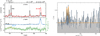 |
Fig. B.1 Left: ISO-LWS and PACS spectra from α Orionis (top, LWS in red) and µ Cephei (bottom, only LWS), after removal of the stellar continua and with identifications of the dominant spectral lines. The LWS spectrum is scaled such that the area under its CO (J = 17 → 16) line corresponds to that of the PACS spectrum. Toward µ Cephei, an off-target spectrum is shown in blue. The green histogram (with vertical offset for better visualization) represents the difference spectrum (with ±1σrms errorbars in selected spectral channels), along with a six-component fit to the CO (J = 18 → 17) and [O I] λ 145.5 μm profiles (in orange). Right: Reprocessed [CII] λ 157.7 μm spectrum from upGREAT’s low-frequency array (dark-gray histogram: central pixel with two-component line fit in orange; bright-gray histogram: average spectrum from off-center pixels). |
We therefore refrained from using the ISO-LWS spectrum for the [C II] λ 157.7 µm line area and prefer the chopped upGREAT observations, despite the weakness of their detection. After adjusting (by a correlation analysis) the total power levels in the average on- and off-target signal of the off-center pixels, the interstellar [C II] λ 157.7 µm emission from µ Cephei canceled out (Fig. B.1). For the central pixel, the same analysis yields, at 3.85 km s−1 velocity resolution, a tentative doublepeak profile with 2.9 and 3.2 σrms detections in the blue- and red-shifted component, respectively. While their separation by (19.5 ± 2.9) km s−1 is not unreasonable, given the low significance we only used the resulting line area, which amounts to (0.11 ± 0.02) × 10−19 W cm−2 in the instrument’s main beam, 14" wide at half-power.
In view of the diverse instrumentation used for the fine-structure line analysis at hand, we conclude this excursion with a benchmark test against the λ63.2 µm and λ158 µm emissions from [OI] and [C II], respectively, from a series of Herbig Ae/Be stars serving as spatially equally unresolved secondary calibrators, using archival ISO (LWS), Herschel (PACS and the Heterodyne Instrument for the Far-Infrared, HIFI), and SOFIA/upGREAT (LFA, HFA) data (Table B.1. The agreement between the [O I] λ 63.2 µm line fluxes from their disk emissions, as measured with the HFA and PACS or LWS, is generally within the quoted uncertainties. For DG Tau A, we note discrepancies between the LWS and PACS/HFA, and between PACS and LWS/HFA for HD 100546. The former can be readily understood as a contamination by DG Tau B in the large ISO/LWS beam (half-power equivalent width 1′.2, Gry et al. 2003). Whether the discrepancy toward HD 100546 is a signpost of line-flux variability caused by a 25 - 50 MJup planet (yet to be confirmed, Blakely et al. 2025) or a hypothetical inner binary companion of subsolar mass (Norfolk et al. 2022) is pure speculation at the present time. We notice the order-of-magnitude discrepancy between the [C II] λ 157.7 µm line flux as measured with ISO/LWS and SOFIA/LFA. It can be readily attributed to a contamination of the LWS spectrum by emissions from CO and CS.
Fine-structure line fluxes of calibrators.
Appendix C Corrections for photochemistry and continuum fluxes
The work presented in the main part of this paper identifies two models (referred to as A and B) offering, within the global uncertainties, concordant solutions for the observed line ratios. The continuum fluxes (Table C.1) are better matched by model A (higher chromospheric temperature, but lower density, than B), but remain uncertain. Regarding the spectral line calibration, the uncertainties of the line area fluxes in [O I] λ 145.5 µm and [C II] λ 157.7 µm are largest. The observed line ratios can be reproduced exactly, if the selected elemental surface abundances (Table A.1) are modified. Model A matches the observed [C II]λ 158 flux only if all carbon residing in C I and CO is photo-chemically converted into C II, and if the elemental carbon abundance is increased by 42%. This would push the C/O ratio from 0.35 (by number) to 0.49, which is not unreasonably far from the prediction of the evolutionary tracks of Ekström et al. (2012, C/O = 0.39, without rotation). We note that a more conservative increment of the elemental carbon abundance would still reproduce the observed [O I]λ 63 /[C II]λ 158 line flux ratio within errors. Model B requires lower (and, for the [C II]λ 158 line flux, less extreme) contributions from photo-chemistry, but overpredicts the [Fe II]λ 26 line flux. This can be corrected by a moderate decrease of the Fe II abundance by 8.4%, which seems reasonable in view of the uncertain elemental Fe abundance. For model A, the good agreement between the observed and modeled [Fe II]λ 26 line fluxes can then be preserved by invoking more photo-ionization of Fe I, which would be a natural consequence of the hotter chromosphere of this model. The results are summarized in Table C.2.
Observed and modeled free-free radio fluxes (top) and dustcontinuum FIR fluxes (bottom).
Appendix D Thermal balance in an expanding dusty envelope
Thanks to the high densities in our models, infrared pumping of the fine-structure level populations by dust emissions can be neglected compared to collisional pumping. Therefore the dust temperature impacts the excitation modeling only through the computation of the dust condensation radius and the resulting dust opacity, which matters for the [S I]λ 25 and [Fe II]λ 26 lines. A proper calculation of the dust temperature profile is thus not indispensable for the analysis at hand. In the following we assess our assumption that the dust condensation radius is approximately given by the gas temperature and pressure. For this purpose we review the thermal balance in the inner envelope of µ Cephei.
Abundance corrections cγ for photochemistry contributions to yields from thermal equilibrium chemistry (indexed TE), required for exactly matching the observed line ratios.
At the dust condensation zone, the gas is mainly heated by collisions with dust grains. Because we consider a region far enough from chromospheric shocks, we neglect heating by photo-electrons from the ionization of atomic carbon and from UV-exposed dust grains4. The heating rate Γ is then given by (e.g., Scoville et al. 1975, equation 7a)
 (D.1)
(D.1)
where nd is the number density of dust grains, σd their crosssection, υD their drift velocity relative to the gas, and ∆T the difference between the dust and gas temperatures. For υD, we refer the reader to equations (6) to (8) of Crosas & Menten (1997), using a description given by Kwok (1975). The underlying stellar luminosity and mass-loss rate are given in Table 2; for the momentum transfer parameter (i.e., the ratio of the cross-section for the radiation pressure and the geometric crosssection) we use that of olivine, computed by Gilman (1974) as a function of grain size and temperature. Γ is then determined across the size distribution of interstellar grains (Mathis et al. 1977, hereafter MRN), such that
 (D.2)
(D.2)
which yields, with lower and upper grain size cutoffs as given by MRN (amin = 5 nm and amax = 250 nm, respectively), ndσd = 1.515 nH · 10−22 cm2, where nH is the hydrogen nucleus number density.
The gas heating is balanced by line cooling and the adiabatic cooling of the expanding gas. The former can be expressed in several ways. Here the underlying level populations are available from the detailed balancing calculations, and the most convenient expression for the line cooling rate is given by Crosas & Menten (1997) through the rates of collisional excitation and de-excitation between levels i and j, Cij and Cji, respectively:
 (D.3)
(D.3)
where the outer sum extends over all levels of an (N + 1) level system except the ground state k = 0.
The line cooling by rotational CO lines is difficult to evaluate. Close to the photosphere, its level population in the vibrational ground state is affected by infrared pumping (through the v = 1 level, 3048 K or λ4.72μm above ground, e.g., Al-Shaqsi et al. 2025). For Betelgeuse, Rodgers & Glassgold (1991) parameterize the CO excitation modeled by Huggins (1987) and demonstrate that in the inner envelope rotational CO line cooling is unimportant compared to fine-structure line (fsl) cooling. Furthermore, our results (section 5 and Table C.2) suggest that CO is underassociated, owing to the chromospherically driven photo-chemistry, as already inferred for Betelgeuse by Huggins (1987). We therefore assume that the fine-structure emissions of O I and C II dominate the line cooling. In model A, the [O I]λ 63 and [O I]λ 145 lines are more important than the [C II]λ 158 line, and vice versa in model B, but with a smaller difference between the two coolants (Fig. D.1).
The adiabatic cooling of a circumstellar envelope of gas temperature Tk expanding at a speed υ(r) and almost fully molecular in the region of interest is given by
 (D.4)
(D.4)
(Goldreich & Scoville 1976). Balancing the resulting heating and cooling rates, Γ = Λ(fsl) + Λ(ad), yields an estimate ∆T for the difference between the dust and gas temperatures. With at most 26 K, it is smaller than the temperature difference between successive grid points, and can be used to determine the distance from the star at which the dust condenses out, as shown in Fig. D.1. This distance, rd(sub), can also be defined through the corresponding thermal equilibrium condition for dust grains of absorption efficiency  , which reads, in the non-gray case and using equations D.1 and D.2,
 (D.5)
(D.5)
with the dilution factor
 (D.6)
(D.6)
Setting Td to the sublimation temperature will define rd; here we refrain from using this approach because the mean intensity of the dust radiation field, Jν is not known without a dedicated dust radiative transfer model of the entire dusty circumstellar envelope (i.e., extending beyond the region that is required for the modeling of the atomic fine-structure line emissions).
Appendix E Ray-tracing and line formation in a spherically symmetric atmosphere
E.1 Numerical solution
The formal solution of the radiative-transfer equation, for a sightline of length L and expressed as Rayleigh-Jeans equivalent line temperature Tℓ, reads
 (E.1)
(E.1)
where Σν and κν are the frequency-specific source function and absorption coefficient, respectively. The parameter study at hand requires an efficient numerical solution of equation E.1, which is detailed in the following. For brevity, we omit the frequency subscripts, but keep in mind that κ is velocity dependent as per the line-profile function. Referring to L as the length of a sightline element sufficiently small to display monotonic first derivatives in Σ and κ, we defined local, second-order approximations to Σ(z) and κ(z), such that
 (E.2)
(E.2)
Partial integration and introducing the expansion
 (E.3)
(E.3)
allows one to express Tℓ in terms of the coefficients pi, qi and q̃i,
 (E.4)
(E.4)
Neglecting the slow rotation of RSG, we adopted spherical symmetry, such that for a sightline at impact parameter p the transformation from the sightline distance z to radius r entails a scaling factor for κ,
 (E.5)
(E.5)
where r ≥ p by definition. The singularity at r = p vanishes upon integration of equation E.1, as one can show by expanding the integrand (up to the above scaling factor) into a power series defined in a sufficiently small environment of r = p, and evaluating it by integration in parts (e.g., Courant 1988). For each sightline element, all coefficients were obtained from straightforward χ2 minimization through parabolic regression. The above approach can be extended to the mixed transfer of spectral line and continuum emissions.
E.2 Approximating complex velocity fields
The spherical symmetry of our approach only allows us to consider centro-symmetric expansion and infall, and precludes motions such as rotation or convection. However, a radial velocity profile as defined by equations 3 and 4 can approximate the line profile arising in spatially unresolved observations of an unbalanced mixture of infalling and upwelling gas cells. For a thin shell, such a velocity structure is shown in Fig. E.1. The 2000 nodes used for this description were created with the procedure SpherePoints embedded in the Mathematica computing environment5. All velocities are referred to a constant turbulent width υt (1/e half-width). In the example shown here and following López Ariste et al. (2018), the convection cells are described by a combination of spherical harmonics up to degree 2, with random radial velocities of |υr| ≤ 14υt. The brightness is taken proportional to velocity (see López Ariste et al. 2018, for the physical motivation of this ansatz). The inner circumstellar envelope consists of 50 nested shells, extending from the stellar surface (r = R*) to r = 2.5 R*. The resulting spectral line profile is shown in Fig. E.1, along with a matching line profile arising from a velocity field described by equations 3 and 4, with parameters υr(R*) = 14.0 υt, υr(rd) = 7 υt, υ∞ = −24.7km s−1, and rd = 2.2 R*. This demonstration suggests that a single, spatially unresolved spectral line profile does not necessarily constrain the nature of the velocity field, especially if the signal-to-noise ratio in the secondary peaks or on the shoulder of the emergent line profile is insufficient.
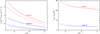 |
Fig. D.1 Left: Fine-structure line cooling rate (solid lines) for models A (red) and B (blue). Dashed and dot-dashed lines show the rates for O I and CII, respectively. Right: Temperature difference ∆T between silicate dust grains (with an MRN size distribution) and the gas, against distance from the stellar center (in units of stellar radii R⋆), for models A (red) and model B (blue). The dashed portions of both lines are for dust temperatures in excess of the stability limit of Forsterite, 1050 K. |
 |
Fig. E.1 Left: Sightline-projected velocity field (VLOS) with pseudo-convective motions in a thin shell, expressed by spherical harmonics. Velocities are measured in units of the intrinsic turbulent width. Right: Surface-integrated spectrum of hypothetical optically thin emission from 50 nested thin shells extending from (1.0–2.5) R⋆. The red spectrum displays the spectrum from the same model without pseudo-convective motions but with a velocity profile defined by equations 3 and 4. |
Appendix F Escape probability from a spherically symmetric extended photosphere
We approximated the non-LTE radiative transfer problem by replacing the non-local coupling of matter and radiation by an escape probability approximation (Sobolev 1957), where the trapping of radiation is accounted for by scaling the Einstein coefficient Ae with the escape probability β(r), given (for a distance r from the center of the star) by
 (F.1)
(F.1)
This expression contains two probabilities; one that a photon is emitted into a direction n at a given velocity offset, as expressed by the line profile function Φ(n, υ), and another one that this photon can escape from the atmosphere (given by the exponential function with the optical depth along the sightline labeled LOS). The radiative coupling between the emitting and the absorbing atom depends on the Doppler shift, the line profile function Φ, and the opacity function κ. For a spherical configuration and a centro-symmetric velocity field (i.e., rotation is neglected), Eq. F.1 becomes
 (F.2)
(F.2)
where θ = 0 and π for sightlines radially directed outward and inward, respectively, and θ* = π–arcsin(R*/r) is the angle between the direction toward the observer and the tangent sightline to the stellar surface. A sketch of the geometry is shown in Fig. F.1. For an analytical solution for a homogeneous sphere expanding at constant velocity we refer to Rybicki & Hummer (1983). The sightlines needed to compute the integral in equation F.2 have equivalent counterparts oriented toward the observer, so that the former can be used to compute the spectral-line flux emerging along the latter sightlines. The radiative-transfer code accounts for this redundancy for speeding up the execution of the calculations; their numerical solution was outlined in Appendix E. We assumed that photons traveling toward the star are not lost but will be absorbed above the photosphere. At the top of the atmosphere, the escape probability for the optically thick case is β(rout) = 0.5, because the photons escape into the outer half-space (we assume that they are not trapped in the outer envelope or astrosphere). In the optically thin limit, the escape probability does not reach unity either because of the assumption of photon trapping toward the star. With these boundary conditions, the escape probability is modified as follows:
 (F.3)
(F.3)
Thanks to the high densities, the excitation modeling converges fast toward solutions close to LTE (three iterations until the relative differences between the escape probabilities from successive iterations differ by less than a factor 10−6). For situations where more than three iterations are needed, we used a linear combination of iterates of β minimizing the residua (Olson et al. 1986), which accelerates the convergence.
Appendix G A spectroscopic distance estimator
Distances to evolved stars are notoriously difficult to measure. To estimate the distance to µ Cephei we are guided here by the physical and spectroscopic similarities between µ Cephei and Betelgeuse and, for the latter source, by the availability of various astrometric and distance estimators. The Hipparcos parallax of Betelgeuse yields  pc (Perryman et al. 1997), corrected later to 152 ± 20 pc (van Leeuwen 2007), but still fraught with systematic uncertainties. Harper et al. (2017) obtained an improved astrometric solution combining the Hipparcos measurements with VLA radio data,
  pc. An independent estimate, combining photometric monitoring with hydrodynamic simulations (Joyce et al. 2020), yields
  pc, differing from, but not incompatible with Harper et al. (2017). Unlike Betelgeuse, µ Cephei has no reliable parallax. Both stars are early-M-type RSGs, as confirmed, for example, by the equivalent width of the CO band head at λ 2.29 µm, known as a temperature estimator for late-type stars (Messineo et al. 2021, further references therein). Moreover, the distances of their warm, molecular layers from the photospheres are comparable, as remarked by Perrin et al. (2005), namely, a third of the respective photospheric diameters. Using for Betelgeuse the original Hipparcos distance of 131 pc and adopting the same photospheric diameters for both stars, they estimated a distance of 390 ± 140 pc. Later, Montargès et al. (2019) used a distance of
  pc, inferred from the update of Betelgeuse’s distance by Harper et al. (2017), and its interferometric K-band diameter (Mon-targès et al. 2014, θκ = 42.28 ± 0.43 mas). Using the same approach, but with a more accurate interferometric angular size of θκ = 16.85 ± 0.15 mas for μ Cephei (Lacour 2010) and for the 168 pc distance to Betelgeuse (Joyce et al. 2020), we obtain for μ Cephei a distance of
  pc (Fig. G.1)6.
 |
Fig. F.1 Sketch of the geometry. The star subtends the red-hatched area. For a given point Q at a distance r from the center of the star, the escape probabilities of photons emitted from Q along the blue sightline segments equal those of photons emitted from Q′ along the green sightline segments toward or away from the observer. |
In view of the large uncertainties of the earlier measurements, and of the potential risk that the photospheric sizes of both stars differ, it is desirable to obtain an independent estimate. Wilson & Vainu Bappu (1957) discovered a tight correlation between absolute visual magnitude (MV) and the logarithmic equivalent widths of the Ca II K emission line, over a 15 mag range in MV. However, in evolved, cool stars, the K-core emission is suppressed by self-absorption arising in their envelopes. Stencel (1977, 1978) showed that in such circumstances, emission lines in the wings of the Ca II H and K lines can be used as an alternative, although for µ Cephei the result remains uncertain. In the same spirit as the Wilson-Bappu effect, Messineo et al. (2021) established tight correlations between photometric luminosities (from GAIA EDR3 parallaxes, Gaia Collaboration 2021) and spectral indices between groups of near-infrared absorption lines from Cr, Fe, Si, Ti, and Mn. High-resolution spectroscopy and accurate parallaxes result in an uncertainty in log L/L⊙ of σ = 0.31 dex. This allows us to take an advantage of reliable GAIA parallaxes, even though unavailable for µ Cephei, and to estimate the luminosity to log(L/L⊙) = 4.98 ± 0.31 dex. Adopting as photospheric temperature the mean temperature of RSGs of type M1, 3780 ± 62K (Arentsen et al. 2019) and with the photospheric K-band diameter (θκ = 16.85 mas, Lacour 2010) at hand, we then infer the distance d (in pc) from the Stefan-Boltzmann law,
![Mathematical equation: \log{d\,\mathrm{[pc]}} = 8.491 + \frac{1}{2}\log{\left(L/L_\odot\right)} - 2\log{T\,\mathrm{[K]}}-\log{\theta_\mathrm{K}\,\mathrm{[mas]}}.](/articles/aa/full_html/2026/07/aa60113-26/aa60113-26-eq45.png) (G.1)
(G.1)
A Monte-Carlo simulation of the resulting distribution using Gaussian random samples in luminosity, photospheric temperature, and radius shows a fairly broad wing extending to ∼1 kpc (Fig. G.1). We note that its third quartile (d = 504 pc) falls well below the 641 pc distance quoted by (Montargès et al. 2019), which we therefore reject.
The two methods are independent from each other, except that they both rely on the measured K-band diameter of µ Cephei. Thanks to its small relative error, the joint probability that either method yields the correct distance can be approximated by the product of the two distributions, which yields  pc, with a photospheric radius of 762R⊙.
 |
Fig. G.1 Probability distributions for distance estimates of µ Cephei. Gray-filled histogram: for spectroscopic luminosity estimate following Messineo et al. (2021). Gray markers indicate the quartiles of the distribution. Salmon-hatched histogram: luminosity estimate from equating the radii of µ Cephei and Betelgeuse (Joyce et al. 2020; Montargès et al. 2014, for the distance and photospheric diameter of the latter, respectively). Blue histogram: joint distribution (the blue marker indicates the median, cyan points delineate a fit by two dimidiated Gaussians). The black marker indicates the distance inferred by Montargès et al. (2019). |
All Tables
Line fluxes for the early-M-type RSG models A and B after corrections for photochemistry (absolute values; ratios with respect to observed fluxes in brackets).
Observed and modeled free-free radio fluxes (top) and dustcontinuum FIR fluxes (bottom).
Abundance corrections cγ for photochemistry contributions to yields from thermal equilibrium chemistry (indexed TE), required for exactly matching the observed line ratios.
All Figures
|
Fig. 1 Fine-structure line emission from µ Cephei, scaled in main-beam brightness temperatures (Rayleigh-Jeans equivalents), as seen in the individual upGreat pixels. Spectra are centered at the pixel positions (median spacings of 34″.4 and 15″.6 for the LFA and the HFA, respectively); Gaussian fits are overlaid in red and spectral baselines in orange. Gray-filled circles indicate the half-power beamwidths of 14″.1 and 6″.6 for the LFA and the HFA, respectively. Left : [OI] λ 63.2 μm emission (HFA, smoothed to 1.2 km s−1 channel spacing.). Right : [CII] λ 157.7 μm emission (LFA, polarization-averaged and smoothed to 9.6 km s−1 channel spacing, see Appendix B and Fig. B.1 for higher resolution). |
| In the text | |
|
Fig. 2 Fine-structure line emission in [O I] λ 63.2 µm (top left), [Fe II] λ 26.0 µm (top right), and [S I] λ 25.2 µm (bottom left, with the telluric H2O feature). Two-component Gaussian fits are overlaid as colored lines and all spectra normalized to unity at peak. Bottom right: zoom into the Gaussian fits (blue: [O I] λ 63.2 µm, red: [Fe II] λ 26.0 µm, green: [S I] λ 25.2 µm). |
| In the text | |
|
Fig. 3 Top: volume-filling factor of the cool clumps (black) and temperature profiles (red) of the early-M-type RSG models A (solid) and B (dashed). Center: densities of selected species from the FASTCHEM simulation, for model A. Bottom: same as the center but for model B. The color code for the displayed species is given in the bottom right corner. Solid lines refer to neutral and dashed lines to singly ionized species. For the definition of models A and B, see Section 4 and Fig. 4. |
| In the text | |
|
Fig. 4 Fine-structure line excitation analysis on a gas densitytemperature grid of early-M-type RSG models, including photochemical enhancement of the [C II]λ158 line flux by a factor 10. Densities and temperatures refer to the location of the chromospheric temperature maximum; blue lines indicate iso-density contours. The colored areas delimit the (ng, Tg) loci where the model-predicted line-area ratios agree with the observed ones within ±1.2σrms: [OI]λ63/[OI]λ145 (Gray), [OI]λ63/[CII]λ158 (cyan), [O I]λ63/[S I]λ25 (red), and [O I]λ63/[Fe II]λ26 (green). The solutions in the red-filled area are compatible with all four measured flux ratios with a 60% likelihood (model A). If the [O I]λ63/[S I]λ25 ratio is omitted, a second solution emerges (model B). The locations of the corresponding least-square solutions are labeled with black dots. The orange abscissa on the top indicates the volume-averaged magnetic field strengths required for virial equilibrium. For details see text. |
| In the text | |
|
Fig. 5 Model spectra of the [O I] λ 63.2 µm line (solid dark blue line for a wind and dashed for inflow) and the [O I] λ 145.5 µm line (light blue), for d = 421 pc and a systemic velocity of υLSR = 36.0 km s−1. The observed λ 63.2 µm spectrum is shown as a gray-filled histogram underneath. Blue arrows mark the systemic velocities discussed in the main text (solid arrow: our model, υLSR = 36kms−1; dashed arrow: υLSR = 32.7 kms−1, Montargès et al. 2021). Model spectra for [CII] λ 157.7 μm, [FeII] λ 26.0 µm, and [S I] λ 25.2 µm are overlaid in black, red, and yellow, respectively. The H I λ 21 cm spectrum (cyan) is scaled, for better visibility. |
| In the text | |
|
Fig. 6 Profiles of radial velocity (red) and of SiO density (the solid blue line is for model A and dashed blue one is for model B). The dark-salmon filled area indicates the velocity range compatible with the range of sightline velocities of SiO (v = 1, J = 2–1) maser components (υLSR = 19 to 43km s−1, Marinho et al. 2024) for a systemic velocity of 36.0 km s−1 (obtained through profile fitting of the [O I]λ63 line). The dotted blue line displays the largest projected distance of v = 1, J = 1–0 SiO maser spots from the star (Colomer 1993, for 421 pc distance). |
| In the text | |
|
Fig. 7 Top left: meridional cuts of line-profile-averaged total optical depths into the envelope (τlos = 0.7 contours where emissions from the inside are attenuated by more than 50%), for model B, with [O I] λ 63.2 µm (dark red), [OI] λ 145.5 µm (bright red), [C II] λ 157.7 µm (black), [FeII] λ 26.0 µm (magenta), and [S I] λ 25.2 µm (gold). Spectral-line opacities dominate the [O I]λ145, [O I]λ63 and [C II]λ 158 transitions, while in [FeII]λ 26 and [S I]λ 25, the λ25 µm continuum opacity prevails. The gray disk represents the extent of the stellar photosphere, the salmon-filled area that of the chromosphere. The sightline to the observer is indicated by the black arrow. Top center to bottom right: contribution functions (i.e., the integrands of Eq. (E.1), normalized to unity at peak) for the respective emissions. |
| In the text | |
|
Fig. B.1 Left: ISO-LWS and PACS spectra from α Orionis (top, LWS in red) and µ Cephei (bottom, only LWS), after removal of the stellar continua and with identifications of the dominant spectral lines. The LWS spectrum is scaled such that the area under its CO (J = 17 → 16) line corresponds to that of the PACS spectrum. Toward µ Cephei, an off-target spectrum is shown in blue. The green histogram (with vertical offset for better visualization) represents the difference spectrum (with ±1σrms errorbars in selected spectral channels), along with a six-component fit to the CO (J = 18 → 17) and [O I] λ 145.5 μm profiles (in orange). Right: Reprocessed [CII] λ 157.7 μm spectrum from upGREAT’s low-frequency array (dark-gray histogram: central pixel with two-component line fit in orange; bright-gray histogram: average spectrum from off-center pixels). |
| In the text | |
|
Fig. D.1 Left: Fine-structure line cooling rate (solid lines) for models A (red) and B (blue). Dashed and dot-dashed lines show the rates for O I and CII, respectively. Right: Temperature difference ∆T between silicate dust grains (with an MRN size distribution) and the gas, against distance from the stellar center (in units of stellar radii R⋆), for models A (red) and model B (blue). The dashed portions of both lines are for dust temperatures in excess of the stability limit of Forsterite, 1050 K. |
| In the text | |
|
Fig. E.1 Left: Sightline-projected velocity field (VLOS) with pseudo-convective motions in a thin shell, expressed by spherical harmonics. Velocities are measured in units of the intrinsic turbulent width. Right: Surface-integrated spectrum of hypothetical optically thin emission from 50 nested thin shells extending from (1.0–2.5) R⋆. The red spectrum displays the spectrum from the same model without pseudo-convective motions but with a velocity profile defined by equations 3 and 4. |
| In the text | |
|
Fig. F.1 Sketch of the geometry. The star subtends the red-hatched area. For a given point Q at a distance r from the center of the star, the escape probabilities of photons emitted from Q along the blue sightline segments equal those of photons emitted from Q′ along the green sightline segments toward or away from the observer. |
| In the text | |
|
Fig. G.1 Probability distributions for distance estimates of µ Cephei. Gray-filled histogram: for spectroscopic luminosity estimate following Messineo et al. (2021). Gray markers indicate the quartiles of the distribution. Salmon-hatched histogram: luminosity estimate from equating the radii of µ Cephei and Betelgeuse (Joyce et al. 2020; Montargès et al. 2014, for the distance and photospheric diameter of the latter, respectively). Blue histogram: joint distribution (the blue marker indicates the median, cyan points delineate a fit by two dimidiated Gaussians). The black marker indicates the distance inferred by Montargès et al. (2019). |
| In the text | |
Current usage metrics show cumulative count of Article Views (full-text article views including HTML views, PDF and ePub downloads, according to the available data) and Abstracts Views on Vision4Press platform.
Data correspond to usage on the plateform after 2015. The current usage metrics is available 48-96 hours after online publication and is updated daily on week days.
Initial download of the metrics may take a while.