| Issue |
A&A
Volume 669, January 2023
|
|
|---|---|---|
| Article Number | A76 | |
| Number of page(s) | 11 | |
| Section | Stellar atmospheres | |
| DOI | https://doi.org/10.1051/0004-6361/202244503 | |
| Published online | 13 January 2023 | |
The effect of winds on atmospheric layers of red supergiants
I. Modelling for interferometric observations★
1
European Southern Observatory (ESO),
Karl Schwarzschildstrasse 2,
85748
Garching bei München, Germany
e-mail: gemma.gonzalezitora@eso.org
2
Astrophysics Research Institute, Liverpool John Moores University,
146 Brownlow Hill,
Liverpool
L3 5RF, UK
3
LUPM, Université de Montpellier, CNRS,
34095
Montpellier, France
4
Max Planck Institute for extraterrestrial Physics,
Giessenbachstrasse 1,
85748
Garching bei München, Germany
Received:
15
July
2022
Accepted:
26
October
2022
Context. Red supergiants (RSGs) are evolved massive stars in a stage preceding core-collapse supernova. The physical processes that trigger mass loss in their atmospheres are still not fully understood, and they remain one of the key questions in stellar astrophysics. Based on observations of α Ori, a new semi-empirical method to add a wind to hydrostatic model atmospheres of RSGs was recently developed. This method can reproduce many of the static molecular shell (or ‘MOLsphere’) spectral features.
Aims. We used this method of adding a semi-empirical wind to a MARCS model atmosphere to compute synthetic observables, comparing the model to spatially resolved interferometric observations. We present a case study to model published interferometric data of HD 95687 and V602 Car obtained with the AMBER instrument at the Very Large Telescope Interferometer (VLTI).
Methods. We computed model intensities with respect to the line-of-sight angle (µ) for different mass-loss rates, spectra, and visibilities using the radiative transfer code TURBOSPECTRUM. We were able to convolve the models to match the different spectral resolutions of the VLTI instruments, studying a wavelength range of 1.8–5 µm corresponding to the K, L, and M bands for GRAVITY and MATISSE data. The model spectra and squared visibility amplitudes were compared with the published VLTI/AMBER data.
Results. The synthetic visibilities reproduce observed drops in the CO, SiO, and water layers that are not shown in visibilities based on MARCS models alone. For the case studies, we find that adding a wind onto the MARCS model with simple radiative equilibrium dramatically improves the agreement with the squared visibility amplitudes as well as the spectra, with the fit being even better when applying a steeper density profile than predicted from previous studies. Our results reproduce observed extended atmospheres up to several stellar radii.
Conclusions. This paper shows the potential of our model to describe extended atmospheres in RSGs. It can reproduce the shapes of the spectra and visibilities with a better accuracy in the CO and water lines than previous models. The method can be extended to other wavelength bands for both spectroscopic and interferometric observations. We provide temperature and density stratifications that succeed, for the first time, in reproducing observed interferometric properties of RSG atmospheres.
Key words: stars: atmospheres / stars: massive / stars: evolution / stars: fundamental parameters / supergiants / stars: mass-loss
Full spectral resolution models are only available at the CDS via anonymous ftp to cdsarc.cds.unistra.fr (130.79.128.5) or via https://cdsarc.cds.unistra.fr/viz-bin/cat/J/A+A/669/A76
© The Authors 2023
 Open Access article, published by EDP Sciences, under the terms of the Creative Commons Attribution License (https://creativecommons.org/licenses/by/4.0), which permits unrestricted use, distribution, and reproduction in any medium, provided the original work is properly cited.
This article is published in open access under the Subscribe-to-Open model. Subscribe to A&A to support open access publication.
1 Introduction
Stellar winds impact the lives of massive stars and can change their evolutionary path in the Hertzprung-Russell diagram (HRD). These mass-loss events become important as the star leaves the main sequence phase (Chiosi & Maeder 1986). For this reason, one of the key stages for mass loss is the red super-giant (RSG) phase, where the massive star is in a stage preceding core-collapse supernova. These mass-loss events occur in the extended atmospheres of RSGs, whose extensions go up to several stellar radii. Beyond that, the temperature is low enough to produce a dusty shell. However, the observed extensions are not at all reproduced by current dynamic model atmospheres which include pulsation and convection (Arroyo-Torres et al. 2015).
As a consequence, the mechanism that triggers mass loss in the extended atmospheres of RSGs is still poorly understood. This is not the case for their low- and intermediate-mass counterparts (Miras), whose mass-loss processes can be explained by pulsation and dust-driven winds alone (Wood 1979; Bowen 1988; Höfner & Olofsson 2018). There have been several attempts to explain the mechanism of stellar winds in RSGs (e.g. Josselin & Plez 2007; Chiosi & Maeder 1986; Kudritzki & Puls 2000), but there is still no consensus. Recent work by Kee et al. (2021) studied the effect of turbulent atmospheric pressure in initiating and determining the mass-loss rates of RSGs, finding promising results. However, further work is needed to unambiguously determine the dynamical processes that trigger massive stellar wind events in spatially extended atmospheres.
Hence, there have been few studies that explore the mass-loss effect in cool massive stars, with all of them focussing on their spectra. Most explore the mid- and far-IR region, where the dust component is dominant (e.g. Groenewegen et al. 2009; Beasor & Davies 2018; Decin et al. 2006; De Beck et al. 2010). Therefore, the models solely rely on dust modelling, such as DUSTY (Ivezic & Elitzur 1997; Ivezic et al. 1999) or RADMC3D (Dullemond et al. 2012). Recently, Davies & Plez (2021) explored the extension of the atmospheres close to the stellar surface at radii smaller than the inner dust shells in the optical and near-IR. Adding the influence of a stellar wind in the MARCS model atmospheres (Gustafsson et al. 2008), Davies & Plez (2021) expanded the atmosphere up to several stellar radii. Their results naturally explained the presence of a mid-IR excess, as well as the mismatch between temperatures derived from the optical and the IR (Levesque et al. 2005; Davies et al. 2013; González-Torà et al. 2021). They also reproduced many of the features obtained by the addition of a static molecular shell (or ‘MOLsphere’). In short, the work by Davies & Plez (2021) opened a new window to explore the mass-loss rates of cool massive stars.
So far, these models have been constrained by comparison to stellar spectra only. The spectral computation shows the flux integrated over the stellar disk and misses the spatially resolved information. Therefore, if we want a detailed way to study spatially extended stellar atmospheres, we need to use interferometric data. Interferometry uses an array of telescopes to increase the angular resolution of the observations. It is a very powerful tool to study the topography of extended atmospheres in detail, and it has been used widely both for RSGs (e.g. Arroyo-Torres et al. 2013; Wittkowski et al. 2012; Climent et al. 2020; Chiavassa et al. 2022) and Miras (e.g. Wittkowski et al. 2018; Kravchenko et al. 2020). As a consequence, interferometry represents a stronger test for models.
For this work, we employed the approach by Davies & Plez (2021) to extend atmospheres for both spectral and interferometric data. We computed the synthetic visibilities of the models for different mass-loss rates (Ṁ) in the wavelength range of the Very Large Telescope Interferometer (VLTI) instruments (1.8–5 µm), which goes from near-IR to mid-IR. We explored the robustness of the model, and we present a case study for VLTI/AMBER (Petrov et al. 2007) data for the RSGs HD 95687 and V602 Car from the sample by Arroyo-Torres et al. (2015). We have chosen these two targets because they are examples of two stars with different masses and therefore different Ṁ, as well as two distinct luminosities.
This paper is organised as follows: Sect. 2 describes the model used for the present study. The theoretical results from our spatially resolved model atmosphere are presented in Sect. 3, followed by the case study for HD 95687 and V602 Car in Sect. 4. Lastly, we conclude in Sect. 5.
2 Methods
In the absence of models that self-consistently explain winds of RSGs, we added a stellar wind with a constant Ṁ to an initial MARCS model (Gustafsson et al. 2008), following the method by Davies & Plez (2021). These models were then used to calculate both the synthetic spectra and the squared visibility amplitudes (|V|2). This is described in detail in the following sections.
2.1 Models
We started with a MARCS model atmosphere. This code assumes local thermodynamic equilibrium (LTE), hydrostatic equilibrium, and spherical symmetry. We defined a radius grid for the model, allowing us to contain a more extended stratification up to ~8.5 R*, where R* is defined as the radius where the Rosseland opacity τRoss = 2/3. Moreover, for simplicity, we assumed that:
The wind is in LTE. A discussion pertaining to this assumption can be found in Davies & Plez (2021).
The model is 1D, so we assumed spherical symmetry.
To determine the outermost density, we used the mass continuity expression
 (1)
(1)
where ρ and v are the density and velocity as a function of the stellar radial coordinate r, respectively. The wind density ρwind(r) has the following shape proposed by Harper et al. (2001):
 (2)
(2)
where Rmax is the arbitrary outer-most radius of the model, in our case 8.5 R*. The β and γ parameters define the smoothness of the extended wind region and were initially set in the semi-empirical 1D model of α Ori by Harper et al. (2001): βHarp = −1.10 and γHarp = 0.45. In Fig. 1 we show what happens when changing the γ and β parameters that define the density profile. The variations of β mostly influence the smoothness of the density profile close to the stellar surface, while the variations of γ influence the full density profile to upper or lower values. We discuss the implications on spectra and interferometric visibility values in Sect. 3.2.1.
The velocity profile was found assuming a fiducial wind limit of v∞ = 25 ± 5 km s−1, that is the value matched to Richards & Yates (1998); van Loon et al. (2005) and Beasor & Davies (2017), and Eq. (1). We assumed no velocity gradient since the acceleration region is shallow and v∞ is due to turbulent motions (see Davies & Plez 2021). The model is sensitive to the density ρ, meaning that  and v are degenerate with one another.
For the temperature profile, we first used simple radiative transfer equilibrium (R.E.), defined as follows:
 (3)
(3)
where T(τRoss=2/3) and R* are the temperature and radius at the bottom of the photosphere, and T(rwind) and rwind are the temperature and radius of the wind extension, respectively. This results in a smoothly decreasing temperature profile for the extended atmosphere.
In addition, Davies & Plez (2021) defined a different temperature profile in their semi-empirical 1D model of α Ori by Harper et al. (2001), based on spatially resolved radio continuum data. The main characteristic of this profile is a temperature inversion in the chromosphere of the star that peaks at ~1.4 R* and decreases again. ALMA and VLA observations of the RSGs Antares and Betelgeuse by Lim et al. (1998) and O’Gorman et al. (2017, 2020) confirm the presence of such a lukewarm chromospheric temperature inversion, peaking at a radius of 1.3–1.5 R* with a peak temperature of ~3800 K. However, Lim et al. (1998) pointed out that optical and ultraviolet chromospheric signatures required higher temperatures of ~5000 K at similar radii (Uitenbroek et al. 1996). Conversely, modelling spectroscopic and interferometric data of the CO MOLsphere derived gas temperatures of only 2000 K at 1.2–1.4 R* (Ohnaka et al. 2013). O’Gorman et al. (2020) suggest that these components coexist in different structures at similar radii in an inhomogeneous atmosphere, and that they are spatially unresolved by current measurements. Observations at different wavelengths may then be sensitive to different structures of this type.
Following Davies & Plez (2021), in our model setup, we included either a temperature profile in R.E., which may be more relevant for observations of the near-IR MOLsphere, or a temperature profile with a chromospheric temperature inversion which may be more relevant for chromospheric signatures in the optical or ultraviolet or for radio continuum observations.
Once the density, temperature, and velocity profiles were defined, we re-sampled the model to a constant logarithmic optical depth sampling ∆ log(τ), and we used 0.01 < ∆ log(τ) < 0.05. The reasons for this re-sampling are explained in Davies & Plez (2021): if the grid is too finely sampled, rounding errors can occur, leading to numerical difficulties. On the other hand, if the sampling is too coarse, the τλ = 2/3 surface is poorly resolved for strong absorption lines.
Finally, we defined the outer boundary of the model where the local temperature is <800 K, which is reached at ~8.5 R*. Below this temperature, our code is unable to reliably converge the molecular equilibrium. In addition, some species would be depleted to dust grains. Figure 2 shows the density, temperature, velocity, and Rosseland opacity profiles for the example of an extended model with log L/L⊙ = 4.8, Teff = 3500 K, log g = 0.0, M = 15 M⊙, and  M⊙ yr−1.
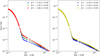 |
Fig. 1 Left: different density profiles for γ = 0.45 and variations of β with β = −1.10 (blue dots), −1.35 (green triangles), and −1.60 (red squares); we noticed that as we decreased β, the wind density near R/R* − 0.99 = 10−1 increased and got steeper. Right: different density profiles for β = −1.10 and the variations of γ with γ = 0.45 (blue dots), 0.25 (black triangles), and 0.05 (yellow squares). In this case, as we increased γ, the slope of the profile remained the same, but the values of the wind density gradually increased. The model used with log L/L⊙ = 4.8, Teff = 3500 K, log g = 0.0, M = 15 M⊙, and |

2.2 Computation of model intensities
We computed both the spectra and the intensity profiles with respect to µ, where µ = cos θ, with θ being the angle between the radial direction and the emergent ray, and cos θ = 1 corresponding to the intensity at the centre of the disk. For this we used the radiative transfer code TURBOSPECTRUM V19.1 (Plez 2012). Setting a wavelength range from 1.8 to 5.0 µm with a step of 0.1 Å, we explored the spectral range of the following instruments at the VLTI:
GRAVITY (GRAVITY Collaboration 2017) for the K band 1.8–2.5 µm.
MATISSE (Lopez et al. 2022) for the L (3.2 < λ < 3.9 µm) and M bands (4.5 < λ < 5 µm). We did not use the N band (8 < λ < 13 µm) because it is dominated by dust emission.
For the spectral synthesis, we included a list of atomic and molecular data. Chemical equilibrium was solved for 92 atoms and their first two ions, including Fe, Ca, Si, and Ti, and molecular data for CO, TiO, H2O, OH, CN, and SiO was included, among about 600 species.
The spectra and visibilities can be convolved to any spectral resolution used by GRAVITY and MATISSE, or instruments at other interferometers. In this work, we show as an example the results convolved to match the HIGH spectral resolution of MATISSE: R = 1000 (available at the CDS).
2.3 Computation of model interferometric visibilities
To compute the visibility from the intensity profile, we used the following Hankel transform as in Davis et al. (2000):
![${V_{{\rm{Model}}}}\left( \lambda \right) = \int_0^1 {{S_\lambda }I_\lambda ^{\rm{\mu }}{J_0}\left[ {\pi {\theta _{{\rm{Model}}}}\left( {B/\lambda } \right){{\left( {1 - {{\rm{\mu }}^2}} \right)}^{1/2}}} \right]{\rm{\mu d\mu }}} ,$](/articles/aa/full_html/2023/01/aa44503-22/aa44503-22-eq8.png) (4)
(4)
where VModel is the visibility of our model, Sλ is the instrument sensitivity curve,  is the computed intensities with respect to µ from TURBOSPECTRUM, J0 is the zeroth order Bessel function, θModel is the angular diameter of the outermost layer of the model, and B is the baseline of the observation. The VModel was then normalised with respect to the total flux.
To estimate θmodel, we used the relation with the Rosseland angular diameter θRoss,
 (5)
(5)
found in Davis et al. (2000) and Wittkowski et al. (2004), where R(τRoss = 2/3) is the radius of the star at τRoss = 2/3, defined as the photospheric layer, and Rmax is the outer most radius of our model.
We used the definition in Wittkowski et al. (2017) to scale the final visibility of the model as
 (6)
(6)
where A allows for the attribution of a fraction of the flux to an over-resolved circumstellar component (Arroyo-Torres et al. 2013), and VModel(θRoss) is the model visibility computed using Eq. (4) with an associated Rosseland angular diameter θRoss from Eq. (5).
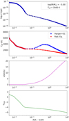 |
Fig. 2 From top to bottom: extended profiles for the density (blue dots), temperature (blue squares for temperature inversion by Harper et al. (2001) also known as ‘Harper’, and red circles for simple radiative equilibrium), wind velocity (purple), and Rosseland optical depth (green). The extended model with log L/L⊙ = 4.8, Teff = 3500 K, log g = 0.0, M = 15 M⊙, |

3 Results
3.1 Base model
We computed the spectra, intensities, and |V|2 for a base model of Teff = 3500 K, log g = 0.0, [Z] = 0, ξ = 5 km s−1, M = 15 M⊙, R* = 690 R⊙, and Rmax = 8.5 R*, corresponding to a RSG similar to HD 95687 (Arroyo-Torres et al. 2015). The density parameters in Eq. (2) are βHarp = −1.10 and γHarp = 0.45 as in Harper et al. (2001) and the wind limit v∞ = 25 km s−1. The temperature profile was initially set to simple R.E., as we are interested in the near-IR K-band MOLsphere (cf. Sect. 2.1). However, we also look at the effect of a chromospheric temperature inversion in Sect. 3.2.2. We used mass-loss rates of  , 10−5, 10−6, and 10−7 M⊙ yr−1, and a simple MARCS model without any wind. As an example, we simulated a star with θRoss = 3 mas, a baseline of B = 60 m, and without any additional over-resolved component, that is A = 1. Figure 3 shows the intensities with respect to the extended stellar radius Rmax for a cut in the continuum (2.26 µm < λ < 2.28 µm), the transition CO (2–0), (λ = 2.29 µm), water (1.9 µm < λ < 2.1 µm), and SiO (λ = 4.0 µm) for the different
  .
.
We observed an extension in all cases except for the MARCS model without the addition of a wind. The CO lines and the SiO lines seem to have the most prominent presence throughout the extended atmosphere (highest intensity compared to water or the continuum). Figures 4–6 show the spectra, the normalised spectra to the continuum, and squared visibility amplitudes (|V|2) computed from our base model with the different  , from highest
  M⊙ yr−1, to the simple MARCS model without wind.
When comparing the spectra and |V|2 in Figs. 4–6, there are several things to notice:
In Figs. 4 and 5, the spectral signatures of CO in the wavelength range of λ = 2.29–2.7 µm (K-band) do not strongly depend on the
 , as they remain relatively unchanged. Only at high
  and high resolution spectra do the low excitation lines start to become stronger, as predicted by Tsuji (1988).
In the region λ > 4.0 µm (L and M bands), the spectra show the presence of SiO lines at wavelengths up to ~4.3 µm, which seem to remain in absorption up to high
 (~10−4 M⊙ yr−1). At ≳4.3 µm we observed the presence of CO as we increased the
  . The CO lines in the M band were already observed in emission at low
  (starting at
  M⊙ yr−1), while the CO at the K band remained in absorption.
In the |V|2 (Fig. 6), the most important thing to notice is that the extended molecular layers, mostly of the CO lines in λ = 2.29–2.7 µm (K-band), are seen in the extended models. This extension was not reproduced earlier with MARCS or PHOENIX (Hauschildt & Baron 1999) models alone.
The CO extension increases with increased
 (in all K, L and M bands). The atmospheric extension is best observed in the M band, as we already see a drop in |V|2 for a low mass-loss rate of
  M⊙ yr−1 (in purple) as compared to a simple MARCS model with no extension (in orange).
The visibility spectra are indicative of extended layers of water vapour (centred at 2.0 µm) for high
 (
( M⊙ yr−1), while the flux spectra are less sensitive. These water features are present in the observations of RSGs (e.g. Arroyo-Torres et al. 2015).
Checking the |V|2, we were not able to reproduce some atomic lines in the 2.10 µm < λ < 2.30 µm region for mass-loss rates
 M⊙ yr−1, which are the most sensitive to the stratification very close to the stellar surface (Kravchenko et al. 2020).
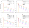 |
Fig. 3 Intensity with respect to the Rmax of our model for simple MARCS (orange), |

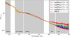 |
Fig. 4 Normalised model spectra with respect to the mean flux for |

3.2 Variations of the base model
3.2.1 Density profile
So far, we have assumed the density parameters (Eq. (2)) from Harper et al. (2001): βHarp = −1.10 and γHarp = 0.45. Figure 7 shows the spectra and |V|2 for the K band for the different β values defined in Fig. 1. We did not include the variations on γ because these produce an almost identical plot. Although the spectra remain unchanged by variations of β the |V|2 change slightly: as the density profile gets steeper (i.e. lower β or γ values), the extension features due to water in λ = 2.35–2.5 µm become more prominent. This can be understood as water layers form close to the stellar surface (Kravchenko et al. 2020), and therefore are sensitive to variations in the density profile in this region. The measurements by Harper et al. (2001) and their constraints of β and γ were less sensitive to the region very close to the stellar surface.
Furthermore, in Fig. 8 we show the spectra in the optical TiO region (λ = 0.5–0.75 µm) to see the effect of changing the β parameter in the TiO lines. Again, changing the γ parameter produces a very similar plot. A discussion concerning the general effect of this semi-empirical model on the TiO bands can be found in Davies & Plez (2021). Briefly, an increase in the mass-loss rate causes the TiO absorption lines to deepen, shifting the star to later spectral types (e.g. for a zero-wind model of spectral type M0, if we apply  , and
, and  M⊙ yr−1 in our model the star is classified as M 1, M 2, and >M 5, respectively). Changing the density profile parameters with a fixed Ṁ affects the TiO bands, also shifting the stellar classification slightly to later spectral types as we deepen the TiO bands (Fig. 8). On the other hand, the TiO bands may be more sensitive to a higher chromospheric temperature component than the molecular layers in the near-IR, which may cause the TiO lines to be less deep (cf. Sect. 2.1).
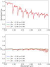 |
Fig. 7 Normalised model spectra (upperpanel) and |V|2 (lower panel) for a fixed γ = 0.45 and the different β = −1.10 (blue), −1.35 (green), and −1.60 (red) in the K-band. The baseline used is B = 63.8 m, corresponding to the case study of HD 95687 in Sect. 4. We can see that as the β gets lower, the water features in λ = 2.35–2.5 µm become slightly more prominent. |
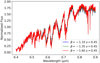 |
Fig. 8 Normalised model spectra for a fixed γ = 0.45 and the different β = −1.10 (blue), −1.35 (green), and −1.60 (red) in the optical TiO band region. As we decrease β, the TiO bands deepen slightly. |
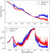 |
Fig. 9 Normalised model spectra (upper panel) and |V|2 (lower panel) for our base model with simple radiative equilibrium (red) and the chromospheric temperature inversion profile by Harper et al. (2001; blue). Both models with a |

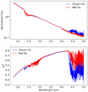 |
Fig. 10 Same as Fig. 9, but with a |

3.2.2 Temperature profile
Figures 9 and 10 show the spectra and |V|2 for our two temperature stratifications defined in Sect. 2, R.E and temperature inversion, with  and
and  M⊙ yr−1, respectively.
When comparing both temperature profiles in Figs. 9 and 10, we see the main difference in the CO lines: in the K-band region λ = 2.29–2.7 µm, the CO is in emission when using the temperature inversion profile (as also predicted by O’Gorman et al. 2020), while for R.E. it remains in absorption even for very high  such as
  M⊙ yr−1. This difference can be seen in the lower panels of Figs. 9 and 10, where the R.E. shows less extension in the CO region as compared with the temperature inversion. For lower mass-loss rates (
 M⊙ yr−1, Fig. 10), it gets harder to see the difference in both profiles. The only region that seems to make a difference is the M band (4.5 < λ < 5 µm), where we see emission in the temperature inversion case.
Observations of CO lines in the K band generally show CO in absorption, even for an extreme case such as the RSG VY CMa (Wittkowski et al. 2012), confirming that the lower temperature based on R.E. is better suited to describe the CO MOLsphere than the higher temperature components of the chromospheric temperature inversion (cf. Sect. 2.1).
To sum up this section, the MARCS+wind model shows significant atmospheric extension in all wavelengths compared to a simple MARCS model (Fig. 3). Such an extension has been observed, but it has so far not been reproduced by current models (Arroyo-Torres et al. 2013). As we increase the  for a R.E. temperature profile, the CO, SiO, and water remain relatively unchanged in the spectra (Fig. 4); whereas for the |V|2, we see a larger extension in all cases (Fig. 6). The R.E. seems to better reproduce the spectra than the temperature inversion as we did not observe the CO in emission in our case studies (see Sect. 4) nor other previously published data (e.g. Wittkowski et al. 2012; Arroyo-Torres et al. 2013, 2015). Changing the β and γ parameters in Eq. (2) deepens the water features in the |V|2.
Parameters of the MARCS models used for the analysis of each RSG.
4 Case study: Comparison with HD 95687 and V602 Car
In this section, we compare our model to published VLTI/AMBER data of the two RSGs HD 95687 and V602 Car available in Arroyo-Torres et al. (2015). As previously mentioned, we have chosen these two RSGs since they sample different luminosities,  , and masses. In addition, the data are readily available, and these are two well-studied RSGs whose fundamental parameters (e.g. Teff, log g, θRoss, and log L/L⊙) are well known. The data were taken using the AMBER medium-resolution mode (R ~ 1500) in the K − 2.1 µm and K − 2.3 µm bands.
The parameters used for each initial MARCS model are shown in Table 1, following Arroyo-Torres et al. (2015). HD 95687 is characterised by a smaller luminosity, mass, and radius than V602 Car. In addition, HD 95687 shows a weaker atmospheric extension than V602 Car.
To estimate both θRoss and A, for each studied model, we computed the |V|2 as a function of their spatial frequency B/λo where λo corresponds to the continuum region 2.23–2.27 µm.
We have compared the model and data |V|2, and found the best-fitting θRoss and A by means of a χ2 minimisation.
Figures 11 and 12 show the MARCS model fit to the data of Arroyo-Torres et al. (2015) and our initial MARCS+wind model fit with βHarp = −1.10 and γHarp = 0.45, compared to the data of HD 95687 and V602 Car, respectively. For our model fit, we checked both the spectra and |V|2. We used a range of mass-loss rates of  with a grid spacing of
  . We obtained a best fit of
  for HD 95687 and
  for V602 Car. These M are reasonable when compared with typical mass-loss prescriptions (e.g. de Jager et al. 1988; Schröder & Cuntz 2005; Beasor et al. 2020).
For the temperature profile, we used R.E. since the temperature inversion would either show depleted CO lines (λ = 2.29–2.7 µm) for the spectra, which do not match with the observations, or not enough extension for the |V|2. Therefore, it is not possible to find a model with the temperature inversion profile that fits both spectra and |V|2 simultaneously.
We estimate for our best-fit models a θRoss = 5.35 ± 0.7 mas and 2.9 ± 0.8 mas, and A = 1.0 ± 0.14 and 1.0 ± 0.08 for V602 Car and HD 95687, respectively. The errors in θRoss and A were derived by the minimum values in the 68% dispersion contours of the χ2 fit, which for 2 degrees of freedom corresponds to  (Avni 1976). Our results are in agreement with Arroyo-Torres et al. (2015) within the error limits.
In this work, we show that when adding a wind to a MARCS model, we are now able to qualitatively fit the spectra and |V|2. This is something that current existing models are unable to do.
This initial fit can be further improved by modifying the inner wind density profile. Figures 13 and 14 show both the spectra and |V|2 of the new fit changing the density parameters in comparison with the data and the initial MARCS+wind fit for HD 95687 and V602 Car, respectively. The main difference between both MARCS+wind models can be found in the |V|2 water region at λ = 2.29–.5 µm, where the new γ and β fit better.
We notice that, although our best-fit model for HD 95687 can accurately reproduce both flux and |V|2, this succeeds for V602 Car to a lower extent: the flux is well reproduced in Fig. 14, but the |V|2 is still missing some extension, especially in the region λ = 2.29–2.5 µm. As previously mentioned, this region not only includes CO, but also the presence of water. A possible explanation for this mismatch could be that for increasing  , the models still fail to reproduce the extension of the water or CO layers. Another possibility is that since our model neglects velocity gradients, it underestimates the equivalent widths of lines. Broader and stronger lines would help to increase the apparent stellar extension at those wavelengths.
5 Summary and conclusion
We present 1D modelling for the extended atmospheres of RSGs based on simple R.E. and chromospheric temperature inversion by Harper et al. (2001), and we computed synthetic flux spectra and synthetic interferometric visibility spectra. When comparing our models to a simple MARCS or PHOENIX models, our synthetic |V|2 showed a stronger atmospheric extension and could fit, for the first time, the observed extension in the case studies.
Regarding the temperature profile, we find that the R.E. reproduces the spectra better than the chromospheric temperature inversion since we do not observe any emission in the CO bands, which are the result of models based on a temperature inversion. The possible reason that R.E. fits better than the temperature inversion – even though RSGs are known to have a chromosphere – could be, on the one hand, because of the presence of different spatial cells with different temperatures in the hot lukewarm chromospheres of RSGs (O’Gorman et al. 2020). On the other hand, we do not know the effect that the dust could make where T > 800 K; although, we expect it to be small.
Moreover, localised gaseous ejections, related to magnetic fields and surface activity were recently suggested as a major contributor to mass loss from RSGs (Humphreys & Jones 2022; Andrews et al. 2022; López Ariste et al. 2022). To explore this effect in detail, we would need to use 3D models, which is out of the scope of this paper. Our 1D modelling approach relies on an azimuthally averaged stratification, which is a good approximation for many aspects, but may not reproduce some of the observed features.
When compared to the observations, we obtain a mass-loss rate that is in accordance with typical mass-loss prescriptions (e.g. de Jager et al. 1988; Schröder & Cuntz 2005; Beasor et al. 2020). However, in order to fit both the water and CO extensions simultaneously, the density shape should be steeper close to the surface of the star than previously expected by Harper et al. (2001).
Most importantly, we were able to reproduce the |V|2 extension of the case studies. Simple stellar atmosphere models such as MARCS do not show extension at all. However, the description very close to the stellar surface may not be optimum yet, as we were not able to reproduce some atomic lines in the 2.10 µm < λ < 2.30 µm |V|2 region, which are the most sensitive to the stratification very close to the stellar surface.
This is the first extended atmosphere model to our knowledge that can reproduce, in great detail, both the spectra and |V|2 simultaneously. Therefore, we have shown the immense potential of this semi-empirical model of MARCS+wind, not only to match the spectral features without the need of dusty shells, but also the visibilities obtained by interferometric means.
In the future, we want to compare this model with data from a wider wavelength range to see the full effects in higher wavelengths such as the L or M bands.
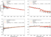 |
Fig. 11 Upper left: normalised flux for the RSG HD 95687 (grey), as observed with VLT/AMBER for the K − 2.1 µm bands. Our initial best-fit model with β = −1.10 and γ = 0.45 is shown in red, corresponding to the parameters of the density profile by Harper et al. (2001). The pure MARCS model fit is shown in orange. As expected, the fluxes are well represented by both our fit and MARCS. Upper right: same as the upper left panel, but for the K − 2.3 µm band. Lower left: same as the upper left panel, but for the |V|2 and a baseline of B = 60.8 m. Lower right: same as the lower right panel, but for the K − 2.3 µm band and a baseline of B = 63.2 m. Our model can represent the data better than simple MARCS. |
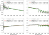 |
Fig. 13 Upper left: normalised flux for the RSG HD 95687 (grey), as observed with VLT/AMBER for the K − 2.1 µm bands. Our initial best-fit model with β = −1.10 and γ = 0.45 is shown in red, corresponding to the parameters of the density profile by Harper et al. (2001). The final best-fit model with β = −1.60 and γ = 0.05 is shown in green. Upper right: same as the upper left panel, but for the K − 2.3 µm band. Lower left: same as the upper left panel, but for the |V|2 and a baseline of B = 60.8 m. Lower right: same as the lower right panel, but for the K − 2.3 µm band and a baseline of B = 63.2 m. The best-fit model for β and γ can reproduce the water features in λ = 2.29–2.5 µm with a better accuracy than our initial best fit. |
Acknowledgements
We would like to thank the anonymous referee for their useful comments which helped to improve paper. Based on observations collected at the European Southern Observatory under ESO programme ID 091.D-0275. GGT is supported by an ESO studentship and a scholarship from the Liverpool John Moores University (LJMU). We want to thank A. Rosales-Guzman and J. Sanchez-Bermudez for useful discussions.
References
- Andrews, H., De Beck, E., & Hirvonen, P. 2022, MNRAS, 510, 383 [Google Scholar]
- Arroyo-Torres, B., Wittkowski, M., Marcaide, J. M., & Hauschildt, P. H. 2013, A&A, 554, A76 [NASA ADS] [CrossRef] [EDP Sciences] [Google Scholar]
- Arroyo-Torres, B., Wittkowski, M., Chiavassa, A., et al. 2015, A&A, 575, A50 [NASA ADS] [CrossRef] [EDP Sciences] [Google Scholar]
- Avni, Y. 1976, ApJ, 210, 642 [NASA ADS] [CrossRef] [Google Scholar]
- Beasor, E. R., & Davies, B. 2017, MNRAS, 475, 55 [Google Scholar]
- Beasor, E. R., & Davies, B. 2018, MNRAS, 475, 55 [NASA ADS] [CrossRef] [Google Scholar]
- Beasor, E. R., Davies, B., Smith, N., et al. 2020, MNRAS, 492, 5994 [Google Scholar]
- Bowen, G. H. 1988, ApJ, 329, 299 [NASA ADS] [CrossRef] [Google Scholar]
- Chiavassa, A., Kravchenko, K., Montargès, M., et al. 2022, A&A, 658, A185 [NASA ADS] [CrossRef] [EDP Sciences] [Google Scholar]
- Chiosi, C., & Maeder, A. 1986, ARA&A, 24, 329 [NASA ADS] [CrossRef] [Google Scholar]
- Climent, J. B., Wittkowski, M., Chiavassa, A., et al. 2020, A&A, 635, A160 [EDP Sciences] [Google Scholar]
- Davies, B., & Plez, B. 2021, MNRAS, 508, 5757 [NASA ADS] [CrossRef] [Google Scholar]
- Davies, B., Kudritzki, R.-P., Plez, B., et al. 2013, ApJ, 767, 3 [Google Scholar]
- Davis, J., Tango, W. J., & Booth, A. J. 2000, MNRAS, 318, 387 [Google Scholar]
- De Beck, E., Decin, L., de Koter, A., et al. 2010, A&A, 523, A18 [NASA ADS] [CrossRef] [EDP Sciences] [Google Scholar]
- de Jager, C., Nieuwenhuijzen, H., & van der Hucht, K. A. 1988, A&AS, 72, 259 [NASA ADS] [Google Scholar]
- Decin, L., Hony, S., de Koter, A., et al. 2006, A&A, 456, 549 [NASA ADS] [CrossRef] [EDP Sciences] [Google Scholar]
- Dullemond, C. P., Juhasz, A., Pohl, A., et al. 2012, Astrophysics Source Code Library [record ascl:1202.015] [Google Scholar]
- González-Torà, G., Davies, B., Kudritzki, R.-P., & Plez, B. 2021, MNRAS, 505, 4422 [CrossRef] [Google Scholar]
- GRAVITY Collaboration (Abuter, R., et al.) 2017, A&A, 602, A94 [NASA ADS] [CrossRef] [EDP Sciences] [Google Scholar]
- Groenewegen, M. A. T., Sloan, G. C., Soszyński, I., & Petersen, E. A. 2009, A&A, 506, 1277 [NASA ADS] [CrossRef] [EDP Sciences] [Google Scholar]
- Gustafsson, B., Edvardsson, B., Eriksson, K., et al. 2008, A&A, 486, 951 [NASA ADS] [CrossRef] [EDP Sciences] [Google Scholar]
- Harper, G. M., Brown, A., & Lim, J. 2001, ApJ, 551, 1073 [NASA ADS] [CrossRef] [Google Scholar]
- Hauschildt, P. H., & Baron, E. 1999, J. Comput. Appl. Math., 109, 41 [NASA ADS] [CrossRef] [Google Scholar]
- Höfner, S., & Olofsson, H. 2018, A&ARv, 26, 1 [Google Scholar]
- Humphreys, R. M., & Jones, T. J. 2022, AJ, 163, 103 [NASA ADS] [CrossRef] [Google Scholar]
- Ivezic, Z., & Elitzur, M. 1997, MNRAS, 287, 799 [Google Scholar]
- Ivezic, Z., Nenkova, M., & Elitzur, M. 1999, Astrophysics Source Code Library [record ascl:9911.001] [Google Scholar]
- Josselin, E., & Plez, B. 2007, A&A, 469, 671 [NASA ADS] [CrossRef] [EDP Sciences] [Google Scholar]
- Kee, N. D., Sundqvist, J. O., Decin, L., de Koter, A., & Sana, H. 2021, A&A, 646, A180 [NASA ADS] [CrossRef] [EDP Sciences] [Google Scholar]
- Kravchenko, K., Wittkowski, M., Jorissen, A., et al. 2020, A&A, 642, A235 [EDP Sciences] [Google Scholar]
- Kudritzki, R.-P., & Puls, J. 2000, ARA&A, 38, 613 [Google Scholar]
- Levesque, E. M., Massey, P., Olsen, K. A. G., et al. 2005, ApJ, 628, 973 [Google Scholar]
- Lim, J., Carilli, C. L., White, S. M., Beasley, A. J., & Marson, R. G. 1998, Nature, 392, 575 [NASA ADS] [CrossRef] [Google Scholar]
- Lopez, B., Lagarde, S., Petrov, R. G., et al. 2022, A&A, 659, A192 [NASA ADS] [CrossRef] [EDP Sciences] [Google Scholar]
- López Ariste, A., Georgiev, S., Mathias, P., et al. 2022, A&A, 661, A91 [NASA ADS] [CrossRef] [EDP Sciences] [Google Scholar]
- O’Gorman, E., Kervella, P., Harper, G. M., et al. 2017, A&A, 602, L10 [NASA ADS] [CrossRef] [EDP Sciences] [Google Scholar]
- O’Gorman, E., Harper, G. M., Ohnaka, K., et al. 2020, A&A, 638, A65 [NASA ADS] [CrossRef] [EDP Sciences] [Google Scholar]
- Ohnaka, K., Hofmann, K. H., Schertl, D., et al. 2013, A&A, 555, A24 [NASA ADS] [CrossRef] [EDP Sciences] [Google Scholar]
- Petrov, R. G., Malbet, F., Weigelt, G., et al. 2007, A&A, 464, 1 [NASA ADS] [CrossRef] [EDP Sciences] [Google Scholar]
- Plez, B. 2012, Astrophysics Source Code Library [record ascl:1205.004] [Google Scholar]
- Richards, A. M. S., & Yates, J. A. 1998, Irish Astron. J., 25, 7 [NASA ADS] [Google Scholar]
- Schröder, K. P., & Cuntz, M. 2005, ApJ, 630, L73 [CrossRef] [Google Scholar]
- Tsuji, T. 1988, A&A, 197, 185 [NASA ADS] [Google Scholar]
- Uitenbroek, H., Dupree, A. K., & Gilliland, R. L. 1996, BAAS, 28, 942 [NASA ADS] [Google Scholar]
- van Loon, J. T., Cioni, M. R. L., Zijlstra, A. A., & Loup, C. 2005, A&A, 438, 273 [NASA ADS] [CrossRef] [EDP Sciences] [Google Scholar]
- Wittkowski, M., Aufdenberg, J. P., & Kervella, P. 2004, A&A, 413, 711 [NASA ADS] [CrossRef] [EDP Sciences] [Google Scholar]
- Wittkowski, M., Hauschildt, P. H., Arroyo-Torres, B., & Marcaide, J. M. 2012, A&A, 540, L12 [NASA ADS] [CrossRef] [EDP Sciences] [Google Scholar]
- Wittkowski, M., Arroyo-Torres, B., Marcaide, J. M., et al. 2017, A&A, 597, A9 [NASA ADS] [CrossRef] [EDP Sciences] [Google Scholar]
- Wittkowski, M., Rau, G., Chiavassa, A., et al. 2018, A&A, 613, L7 [NASA ADS] [CrossRef] [EDP Sciences] [Google Scholar]
- Wood, P. R. 1979, ApJ, 227, 220 [NASA ADS] [CrossRef] [Google Scholar]
All Tables
All Figures
|
Fig. 1 Left: different density profiles for γ = 0.45 and variations of β with β = −1.10 (blue dots), −1.35 (green triangles), and −1.60 (red squares); we noticed that as we decreased β, the wind density near R/R* − 0.99 = 10−1 increased and got steeper. Right: different density profiles for β = −1.10 and the variations of γ with γ = 0.45 (blue dots), 0.25 (black triangles), and 0.05 (yellow squares). In this case, as we increased γ, the slope of the profile remained the same, but the values of the wind density gradually increased. The model used with log L/L⊙ = 4.8, Teff = 3500 K, log g = 0.0, M = 15 M⊙, and |
| In the text | |
|
Fig. 2 From top to bottom: extended profiles for the density (blue dots), temperature (blue squares for temperature inversion by Harper et al. (2001) also known as ‘Harper’, and red circles for simple radiative equilibrium), wind velocity (purple), and Rosseland optical depth (green). The extended model with log L/L⊙ = 4.8, Teff = 3500 K, log g = 0.0, M = 15 M⊙, |
| In the text | |
|
Fig. 3 Intensity with respect to the Rmax of our model for simple MARCS (orange), |
| In the text | |
|
Fig. 4 Normalised model spectra with respect to the mean flux for |
| In the text | |
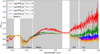 |
Fig. 5 Same as Fig. 4, but for the flux normalised to the continuum. |
| In the text | |
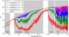 |
Fig. 6 Same as Fig. 4, but for the modelled visibility |V|2. The baseline assumed is B = 60 m. |
| In the text | |
|
Fig. 7 Normalised model spectra (upperpanel) and |V|2 (lower panel) for a fixed γ = 0.45 and the different β = −1.10 (blue), −1.35 (green), and −1.60 (red) in the K-band. The baseline used is B = 63.8 m, corresponding to the case study of HD 95687 in Sect. 4. We can see that as the β gets lower, the water features in λ = 2.35–2.5 µm become slightly more prominent. |
| In the text | |
|
Fig. 8 Normalised model spectra for a fixed γ = 0.45 and the different β = −1.10 (blue), −1.35 (green), and −1.60 (red) in the optical TiO band region. As we decrease β, the TiO bands deepen slightly. |
| In the text | |
|
Fig. 9 Normalised model spectra (upper panel) and |V|2 (lower panel) for our base model with simple radiative equilibrium (red) and the chromospheric temperature inversion profile by Harper et al. (2001; blue). Both models with a |
| In the text | |
|
Fig. 10 Same as Fig. 9, but with a |
| In the text | |
|
Fig. 11 Upper left: normalised flux for the RSG HD 95687 (grey), as observed with VLT/AMBER for the K − 2.1 µm bands. Our initial best-fit model with β = −1.10 and γ = 0.45 is shown in red, corresponding to the parameters of the density profile by Harper et al. (2001). The pure MARCS model fit is shown in orange. As expected, the fluxes are well represented by both our fit and MARCS. Upper right: same as the upper left panel, but for the K − 2.3 µm band. Lower left: same as the upper left panel, but for the |V|2 and a baseline of B = 60.8 m. Lower right: same as the lower right panel, but for the K − 2.3 µm band and a baseline of B = 63.2 m. Our model can represent the data better than simple MARCS. |
| In the text | |
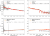 |
Fig. 12 Same as Fig. 11, but for V602 Car. |
| In the text | |
|
Fig. 13 Upper left: normalised flux for the RSG HD 95687 (grey), as observed with VLT/AMBER for the K − 2.1 µm bands. Our initial best-fit model with β = −1.10 and γ = 0.45 is shown in red, corresponding to the parameters of the density profile by Harper et al. (2001). The final best-fit model with β = −1.60 and γ = 0.05 is shown in green. Upper right: same as the upper left panel, but for the K − 2.3 µm band. Lower left: same as the upper left panel, but for the |V|2 and a baseline of B = 60.8 m. Lower right: same as the lower right panel, but for the K − 2.3 µm band and a baseline of B = 63.2 m. The best-fit model for β and γ can reproduce the water features in λ = 2.29–2.5 µm with a better accuracy than our initial best fit. |
| In the text | |
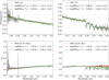 |
Fig. 14 Same as Fig. 13, but for V602 Car. |
| In the text | |
Current usage metrics show cumulative count of Article Views (full-text article views including HTML views, PDF and ePub downloads, according to the available data) and Abstracts Views on Vision4Press platform.
Data correspond to usage on the plateform after 2015. The current usage metrics is available 48-96 hours after online publication and is updated daily on week days.
Initial download of the metrics may take a while.