


| Issue |
A&A
Volume 711, July 2026
|
|
|---|---|---|
| Article Number | A183 | |
| Number of page(s) | 16 | |
| Section | Galactic structure, stellar clusters and populations | |
| DOI | https://doi.org/10.1051/0004-6361/202659704 | |
| Published online | 14 July 2026 | |
Low-resolution spectroscopic characterisation of five poorly known Galactic stellar clusters
1
Kapteyn Astronomical Institute, University of Groningen,
Landleven 12,
9747
AD
Groningen,
The Netherlands
2
Dipartimento di Fisica e Astronomia “Augusto Righi”, Università di Bologna,
Via Gobetti 93/2,
40129
Bologna,
Italy
3
INAF – Osservatorio di Astrofisica e Scienza dello Spazio di Bologna,
Via Gobetti 93/3,
40129
Bologna,
Italy
4
INAF – Osservatorio Astronomico di Padova,
Vicolo dell’Osservatorio 5,
Padova
35122,
Italy
5
Institute for Computational Cosmology & Centre for Extragalactic Astronomy, Department of Physics, Durham University,
South Road,
Durham
DH1 3LE,
UK
★ Corresponding author: This email address is being protected from spambots. You need JavaScript enabled to view it.
Received:
4
March
2026
Accepted:
2
June
2026
Abstract
Stellar clusters preserve crucial information on the formation and evolutionary processes that shaped the Milky Way (MW) as we see it today. However, several MW clusters still lack sufficient data to constrain their metallicity, ages, and, in some cases, even their basic kinematic properties. We present low-resolution MODS at LBT spectroscopy for five such systems (i.e. Koposov 1, Koposov 2, Muñoz 1, Pfleiderer 2, and RLGC2) from which we derive systemic heliocentric radial velocities (Vsys) with typical uncertainties of ≤10 km s−1, and metallicities based on the equivalent widths of the infrared Ca II triplet measured in red giant branch members. For Pfleiderer 2 and RLGC2, we provide the first spectroscopic determinations of their systemic velocities and metallicities, for which we find Vsys = 6 ± 5 km s−1 and −313 ± 6 km s−1, and [Fe/H] = −0.75 ± 0.09 dex and −2.33 ± 0.13 dex, respectively. For the other three clusters, we find results that are consistent with the existing literature. Thanks to our new spectroscopic measurements, we were able to perform an orbital analysis to investigate their origin. We find that Pfleiderer 2 likely formed within the MW, RLGC2 is dynamically associated to the Gaia–Sausage–Enceladus accretion event, and Koposov 1 was likely stripped from the Sagittarius dwarf spheroidal while Muñoz 1 is only tentatively associated with the latter system. Koposov 2, at a high orbital energy, does not show a clear association with any known progenitor system.
Key words: stars: abundances / stars: kinematics and dynamics / Galaxy: evolution / globular clusters: general
© The Authors 2026
 Open Access article, published by EDP Sciences, under the terms of the Creative Commons Attribution License (https://creativecommons.org/licenses/by/4.0), which permits unrestricted use, distribution, and reproduction in any medium, provided the original work is properly cited.
This article is published in open access under the Subscribe to Open model. This email address is being protected from spambots. You need JavaScript enabled to view it. to support open access publication.
1 Introduction
Globular clusters (GCs) are among the oldest stellar systems in the Galaxy and have long been regarded as pristine fossils of its early assembly (Searle & Zinn 1978). The discovery and characterisation of the accreted population of GCs in the Galaxy (e.g. Forbes & Bridges 2010; VandenBerg et al. 2013; Massari et al. 2019; Horta et al. 2020; Callingham et al. 2022; Ceccarelli et al. 2024; Chen & Gnedin 2024; Monty et al. 2024; De Leo et al. 2026b), observations of massive bound clusters forming at high redshift (Vanzella et al. 2017; Claeyssens et al. 2023; Adamo et al. 2024), and the growing evidence that a large fraction of the early Milky Way (MW) may have formed within (now disrupted) GCs (Schiavon et al. 2017; Belokurov & Kravtsov 2023) are just a few examples that highlight their crucial role in the assembly and early chemical enrichment of galaxies. However, a significant fraction of the MW GCs system is, essentially, unexplored to date. Even though the population of massive, high-luminosity GCs in the Galactic halo is now close to being fully inventoried (see e.g. Webb & Carlberg 2021), a growing number of low-mass and low-surface-brightness stellar systems have been discovered in the last two decades (e.g. Belokurov et al. 2010; Fadely et al. 2011; Minniti et al. 2011; Laevens et al. 2015; Kim et al. 2016; Koposov et al. 2017; Garro et al. 2020; Gran et al. 2022). Their physical properties often place them in a transitional regime where traditional classifications between GCs and more diffuse stellar systems (e.g. ultra-faint dwarf galaxies, open clusters) are no longer clear-cut (Conn et al. 2018; Muñoz et al. 2018; Mau et al. 2020). Moreover, many of these clusters are observationally challenging, either residing in the far reaches of the MW halo or buried behind heavy extinction towards the Galactic disc and bulge (Massari et al. 2025). This means that some of the most intriguing clusters still lack even basic spectroscopic characterisation, including their systemic heliocentric radial velocity (Vsys), metallicity ([Fe/H]), and/or [α/Fe] ratio, which limits our ability to constrain their origin, current dynamical state, and evolution. To partially address this gap, we collected low-resolution spectra for five systems observed by the Hubble Missing Globular Cluster Survey (MGCS, Massari et al. 2025), namely Koposov 1, Koposov 2, Muñoz 1, Pfleiderer 2, and RLGC2, that are either heavily extinct and/or very sparse and distant (Koposov et al. 2007; Ortolani et al. 2009; Muñoz et al. 2012; Ryu & Lee 2018). By targeting the brightest accessible stars, we aim to obtain robust measurements of the clusters’ systemic velocities and, whenever possible, to derive their spectroscopic metallicity, based on the equivalent width (EW) of the infrared Ca II triplet. For Koposov 1, Koposov 2, and Muñoz 1, our analysis provides an independent validation of literature results (Muñoz et al. 2012; Cerny et al. 2026; Geha et al. 2026), while for Pfleiderer 2 and RLGC2 we provide the first ever spectroscopic measurements. Together, these observations complement MGCS data and supply the necessary kinematic and chemical information required to place these stellar clusters in a chemo-dynamical framework, and to better constrain their role within the assembly history of the MW.
Information on the observations for target clusters.
2 Observations and data reduction
All target clusters were observed with the low-resolution MultiObject Double Spectrographs (MODS, Pogge et al. 2010) at the Large Binocular Telescope (LBT, Programme IT-2024B-009, PI: E. Ceccarelli); see Table 1 for a summary of the observations. MODS is composed of a pair of optical multi-object spectrographs (MODS1 and MODS2) mounted on the two LBT binocular arms. MODS spectra were obtained in dichroic mode using both the G400L (3500–5900 Å) and the G670L (5400–10 000 Å) gratings on the blue and red channels, respectively. Such a wide wavelength range enables the detection of several absorption features that are key for retrieving a precise heliocentric radial velocity (Vlos).
For each cluster we designed a mask containing 0.6″ slits (yielding a spectral resolution of R ~ 2300) for up to seven stars per cluster (all the information is reported in Table A.1) selected according to the proper motion based membership probability (p > 80%) by Vasiliev & Baumgardt (2021). Masks were observed with MODS in dual mode with two exposures of 1200 s each. Due to the presence of a small veil of clouds, Pfleiderer 2 and RLGC2 were observed with one extra exposure.
We reduced the spectra using the Spectroscopic Interactive Pipeline and Graphical Interface (SIPGI) tool (Gargiulo et al. 2022). In particular, we produced calibration frames for both MODS1 and MODS2 following the procedure outlined below. Firstly, we generated a bad pixel map using imaging flats and applied it to every observed frame, together with the correction for the presence of cosmic rays. We independently bias-subtracted and flat-field corrected each frame using a master flat derived from a set of multi-object spectrograph flats. We then applied the dispersion solution to each frame in order to perform the wavelength calibration and correct for optical distortions. To do so, we used a master lamp obtained from a series of arc lamp exposures. Using SIPGI, we were able to achieve a typical precision in the wavelength calibration of ~10 km s−1 (Gargiulo et al. 2022). We then extracted the two-dimensional, wavelength-calibrated spectra and performed the sky subtraction. Finally, we extracted the one-dimensional spectrum of each source and shifted it to the air-calibrated wavelength rest-frame (see e.g. Edlén 1966; Hanuschik 2003). Finally, we applied the heliocentric velocity correction along the line of sight (measured at the time of each corresponding observation with the rvcorrect task from IRAF1) on the spectra of each star, and stacked them together to improve the signal-to-noise (S/N) ratio.
In Fig. 1, we plot the Gaia colour-magnitude diagram (CMD) obtained from the catalogue by Vasiliev & Baumgardt (2021) for Pfleiderer 2, together with the highest and lowest S/N stellar spectra, to show the quality of the data around some absorption features of interest, i.e. Hα and Ca II triplet (CaT). The same plots for all clusters are in Appendix A.
3 Chemodynamical analysis
In this section, we present the details of the analysis performed on the spectra. The discussion and interpretation of the results are deferred to Section 4.
3.1 Heliocentric radial velocity
For each star, we measured the Vlos using the fxcor task from IRAF, which implements the cross-correlation method described in Tonry & Davis (1979). As template spectra, we used synthetic spectra generated with the code SYNTHE (Kurucz 2005) and adopted new ATLAS9 model atmospheres based on the KOALA database (Mucciarelli et al. 2026).
The atmospheric parameters used to generate the synthetic spectra were derived as follows and are listed in Table A.1:
Metallicity ([Fe/H]): we adopted literature metallicity estimates from isochrone fitting for Pfleiderer 2 ([Fe/H] = 0.0 dex, Ortolani et al. 2009) and RLGC2 ([Fe/H] = −2.1 dex, Ryu & Lee 2018). For Koposov 1, Koposov 2, and Muñoz 1, we adopted [Fe/H] = −0.9 dex, [Fe/H] = −2.9 dex, and [Fe/H] = −1.4 dex, respectively, as previously derived from spectra obtained with the DEep Imaging MultiObject Spectrograph (DEIMOS) at Keck (Muñoz et al. 2012; Cerny et al. 2026; Geha et al. 2026).
Effective temperature (Teff): we relied on colour - Teff relations from Mucciarelli et al. (2021) to derive the effective temperatures using the Gaia (BP − RP) colour (Gaia Collaboration 2023). Since the adopted colour − Teff relation depends on the metallicity of the star (Mucciarelli et al. 2021), the [Fe/H] listed above were initially assumed to estimate first-order temperature, which were subsequently refined using the spectroscopic metallicities obtained in this work (see Section 3.3).
Surface gravity (log g): we estimated the log g starting from the Stefan-Boltzmann relation; we adopted the Teff obtained photometrically and assumed a stellar mass of M⋆ = 0.8 M⊙, which is representative for evolved stars in old GCs, as indicated by theoretical stellar evolution models (Hidalgo et al. 2018; Pietrinferni et al. 2021).
For the stars with a S/N > 10 around both the Hα line and the CaT lines, the Vlos was derived through a single cross-correlation with a synthetic spectrum with proper atmospheric parameters, performed over the full wavelength range and masking the portions of the spectrum affected by telluric absorptions. However, this approach proved problematic for the two brightest stars in Muñoz 1. As horizontal branch stars (see Fig. A.2), their spectra are heavily contaminated by hydrogen Paschen lines within the CaT region, which compromise the velocity fit. Therefore, for these two stars and for the remaining targets, we only used the Hα line, as the combination of the low S/N ratio and/or the intensity of the CaT lines was insufficient to provide reliable measurements (see Table A.1). The resulting values are reported in Table 2. The uncertainty on the measured Vlos was computed by accounting for two independent contributions. The first term accounts for the precisions achieved with the wavelength calibration (see Section 2). The second term accounts for the quality of the spectrum (i.e. S/N) and is derived from Monte Carlo simulations. For each star, we generated 500 synthetic spectra, adding Poisson noise to match the average S/N of the observed MODS spectrum, and resampled them to the instrumental pixel scale. Then, we computed the cross-correlation functions between these noisy spectra and the corresponding synthetic spectrum using the same procedure adopted for the data (including telluric masking when applicable or restricting the analysis to the Hα region for lower S/N spectra). The 1σ dispersion of the resulting Vlos distribution was taken as this contribution to the uncertainty. These terms were combined in quadrature to obtain the final uncertainty. Final values are reported in Table 2, together with the average systemic heliocentric radial velocity calculated from likely members (see following discussion). We note that we have six stars in common with Geha et al. (2026), two in Koposov 1, three in Koposov 2, and one in Munoz 1, and the Vlos we measure for these stars are always consistent within the uncertainties.
To interpret the results, we compared the kinematics (and metallicity, see Section 3.3) of the observed stars with synthetic Galactic field populations, computed with the Besançon Galaxy Model2 (BGM, Robin et al. 2003). The comparison samples include stars located within 1° of the centre of each cluster and selected in regions of the CMD populated by our stellar targets. We show the results for Pfleiderer 2 in Fig. 2 and for all other targets in Figs. B.1–B.2. For three of the clusters (Koposov 1, Pfleiderer 2, and RLGC2), we find that all targeted stars have heliocentric radial velocities that are consistent among each other within the uncertainties. For Pfleiderer 2 and Koposov 1, the Vsys we measure coincide with the peak of the velocity distribution predicted for the field population by the BGM, and their mean proper motions (see Vasiliev & Baumgardt 2021) are also partially consistent with those of the synthetic field population. Nevertheless, there is an extremely low probability of randomly drawing a number of stars equal to those that define our sample from the BGM distributions, assuming Gaussian uncertainties comparable to the typical measurement errors and simultaneously matching the three-dimensional kinematic properties of the two clusters within the observed ranges (p ~ 3 × 10⁻²⁸ and p ~ 1 × 10⁻¹² for Pfleiderer 2 and Koposov 1, respectively). In contrast, RLGC2 lies well outside both the Vlos and proper motion distributions expected for the field population, which means that virtually no field star is plausibly expected to contaminate our sample. These comparisons strongly indicate that targeted stars are bona fide members of their respective clusters. For both Koposov 2 and Muñoz 1, we find that one out of the four observed stars has a Vlos that is inconsistent with the average of the other three targets (at 3.7σ and 2.5σ, respectively, see hatched histograms in Figs. B.1–B.2). We note that only ~1% of the respective surrounding Galactic field populations have proper motions compatible with those of the clusters. In the case of Koposov 2, the Vsys we measure for the cluster is also offset from the peak of the field-star velocity distribution predicted by the BGM by ~100 km s−1. Interestingly, the star with a different Vlos instead falls close to that peak, which makes it a possible candidate field contaminant. For Muñoz 1, the situation is somewhat different: the cluster systemic velocity lies within the bulk of the field Vlos distribution. Nevertheless, the probability of drawing a contaminant with a velocity comparable to that of the outlier star is only p ~ 1 × 10⁻³. Despite this, Muñoz 1 is an ultra-faint stellar cluster for which a very small intrinsic velocity dispersion is expected (Cerny et al. 2026); therefore, we conservatively exclude this star from the cluster sample. These stars have been marked with a coloured cross in Figs. A.1, A.2, B.1, and B.2. The derived Vsys of Koposov 1, Koposov 2, and Muñoz 1 are measured as the average of the Vlos of likely members. We report values of Vsys = 10 ± 9 km s−1, Vsys = 112 ± 9 km s−1, and Vsys = −127 ± 10 km s−1, respectively, which are fully consistent with those reported in the literature (Muñoz et al. 2012; Geha et al. 2026).
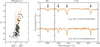 |
Fig. 1 Left panel: Gaia CMD for Pfleiderer 2 from Vasiliev & Baumgardt (2021). Typical photometric errors at these magnitudes can be found in Gaia Collaboration (2021). All stars with a probability of membership >80% are shown in black, while our selected target stars are plotted in orange. A BaSTI isochrone (Hidalgo et al. 2018, 10 Gyr, [Fe/H] = −0.7 dex, solar-scaled [α/Fe]) is also plotted for reference, taking distance and reddening estimates from Ortolani et al. (2009). Right panel: MODS spectra for the highest and lowest S/N stars among our sample, shown around the Hα and CaT regions (the positions of such absorption lines are indicated with arrows). The same plots for other clusters can be found in Appendix A (see Figs. A.1–A.2). |
Photometric atmospheric parameters and results from the spectroscopic analysis.
3.2 Orbital parameters
Thanks to the spectroscopic determination of the Vsys, we are now able to accurately investigate the motion of these clusters within the Galaxy3. In particular, we complemented the Vsys measurements with the full five-dimensional phase-space information, taking positions and proper motions from Gaia data (Vasiliev & Baumgardt 2021) and distances from isochrone fitting (Ortolani et al. 2009; Muñoz et al. 2012; Paust et al. 2014; Ryu & Lee 2018). We note that, for some of these clusters, the distance estimates reported in the literature differ by up to ~15 kpc (see e.g. Koposov et al. 2007; Paust et al. 2014; Muñoz et al. 2018; Cerny et al. 2026; Geha et al. 2026). We therefore discuss in Appendix C how the adopted distance influences the inferred dynamical associations and the derived metallicities. For Koposov 2, Pfleiderer 2, and RLGC2, we adopted proper motions obtained from the combination of Gaia and HST data as provided by the MGCS survey, which allowed measurements with improved precision compared to Gaia alone (Libralato et al. 2026). All the values are listed in Table 3.
To compute the cluster orbits, we adopted a Galactocentric reference frame assuming the solar position and motion to be those defined in Drimmel & Poggio (2018), GRAVITY Collaboration (2018), and Bennett & Bovy (2019). We integrated orbits within the McMillan (2017) MW potential using the AGAMA package (Vasiliev 2019). For each object, we performed 100 Monte Carlo orbit realisations, assuming Gaussian uncertainties in distance, proper motion, and systemic heliocentric radial velocity. Final orbital parameters were taken as the median of the resulting distributions, with associated ±1σ uncertainties. Figure 3 illustrates the location of the clusters in the E–LZ–L⊥ space, compared with the distribution of the full MW GC population (Massari et al. 2019, eDR3 edition)4. To guide the eye, we colour in-situ GCs in black, and we draw two ellipses that highlight the 1σ distributions of GCs formed in the Gaia-Sausage-Enceladus dwarf galaxy (GSE, Belokurov et al. 2018; Helmi et al. 2018) or in the Sagittarius dwarf spheroidal (Sag dSph, Ibata et al. 1994), according to Massari et al. (2019, eDR3 edition). A detailed discussion of the associations of these clusters is presented in Section 4.
To assess the impact of the rotating bar of the MW on the recovered dynamical parameters (and thus on the associations), we redid the integration with the code ORBIT (De Leo et al. 2026a,b). We found that the introduction of the bar in the underlying potential used for the integration produces minimal changes (<10%) in the dynamical parameters of most of the target clusters, and does not alter the associations. Pfleiderer 2 is the exception, being the most impacted by the action of the bar, with changes in the orbital parameters of up to about ~30% (see Section 4).
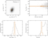 |
Fig. 2 Top row: vector-point diagram (left) for a synthetic Galactic field population (located within 1° from Pfleiderer 2 and selected in the same CMD region populated by the RGB of the cluster) computed with a BGM (Robin et al. 2003). The proper motion of Pfleiderer 2 from Vasiliev & Baumgardt (2021) is indicated with a ‘plus’ marker. On the right panel we display the Vlos distribution of cluster (orange) and field stars from the BGM (grey) as a function of the distance from the cluster centre. Here, stars identified as outliers in Vlos are marked with crosses. Bottom row: heliocentric radial velocity (left) and metallicity (right) distributions for Pfleiderer 2 (orange) and for the BGM synthetic field population (grey). |
3.3 Metallicity from CaT equivalent widths
To measure the EW for each CaT absorption feature (8498.0, 8542.1, and 8662.1 Å), we fitted each line in the normalised spectrum with a Voigt function, thereby accounting for the non-Gaussian profile of their wings. The line centres were fixed to their nominal wavelengths, while all other parameters in the Voigt model were left free during the fit. The EWs were computed by numerically integrating the best-fitting model over the line region. Uncertainties were estimated via Monte Carlo simulations by repeating the measurements over 500 synthetic spectra obtained by adding Poisson noise (according to the S/N of each star). The final EW uncertainty was defined as the 1σ confidence interval of the resulting EW distribution.
To convert EWs into metallicities, we used the recently published calibrations by Navabi et al. (2026), which use the absolute Gaia G magnitude as a luminosity proxy. This choice is driven by the fact that, for the clusters analysed in this work, it is not possible to reliably estimate the apparent magnitude of the horizontal branch due to the lack of multiple stars in this evolutionary sequence. Robust average metallicity estimates based on multiple red giant branch (RGB) stars are only possible for Pfleiderer 2 and RLGC2. For Koposov 1, Koposov 2, and Muñoz 1, our sample included only a single RGB star with sufficient S/N to derive a reliable metallicity. We note that the two brightest stars in Muñoz 1 are significantly hot (Teff > 8800 K) and their CaT spectral region is contaminated by hydrogen Paschen lines (see Fig. A.2), which prevents a reliable metallicity determination. Also, the star used for Muñoz 1 is fainter than MV = 2, and therefore the adopted relations were applied beyond their nominal calibration range. The uncertainties were derived by propagating the errors associated with the EW measurements, the observed magnitudes and distances, as well as the intrinsic uncertainty of the calibration relation (Navabi et al. 2026). All the values are listed in Table 2. In Appendix D, we compare the values derived from the Navabi et al. (2026) calibration with those obtained using alternative relations (Carrera et al. 2007; Starkenburg et al. 2010; Carrera et al. 2013). Such an exercise is aimed at assessing the robustness of the metallicity estimates (see Table D.1).
All three stars in Koposov 1, Koposov 2, and Muñoz 1 for which we are able to measure the metallicity are included in the catalogue published by Geha et al. (2026). For these objects, we find excellent agreement with their reported values, which are [Fe/H] = −1.02 ± 0.15 dex, [Fe/H] = −2.89 ± 0.18 dex, and [Fe/H] = −1.26 ± 0.27 dex, respectively. Furthermore, if we consider the cluster metallicities derived by Cerny et al. (2026), we still obtain values that are consistent with our estimates within the quoted uncertainties for Koposov 2 and Muñoz 1, while we find Koposov 1 to be more metal poor by ~0.4 dex, and not consistent within 2.7σ. When compared with the metallicity distribution of field stars in the surrounding regions of the BGM, we note that only a handful of field stars around Koposov 2 reach such low metallicities (<1% with [Fe/H] < −2.5 dex, see Fig. B.1). Given that Koposov 2 is observed close on the sky to the Sag dSph, it is worth noting that stars with [Fe/H] < −2.0 dex are known to exist in the Sag dSph, although they constitute only a very small fraction of its stellar population (e.g. Mucciarelli et al. 2017; Hayes et al. 2020; Minelli et al. 2023). For Koposov 1, Muñoz 1, and Pfleiderer 2 the probability of finding field stars with comparable metallicities is not negligible, although the average values of the clusters remain offset from the peak of the field stars metallicity distribution. This should nevertheless be considered together with the fact that the likelihood of a field star simultaneously matching the observed proper motion and Vsys is already low (see Section 3.1). Finally, RLGC2 is ~1 dex below the most metal-poor tail of the metallicity distribution of the surrounding stellar population. Therefore, we deem these stars as probable members of each respective cluster.
Five-dimensional phase-space information (position, proper motion, and distance) from the literature for the target clusters.
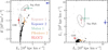 |
Fig. 3 Distribution in the integral-of-motions (E, Lz, L⊥) space of the stellar clusters studied in this paper, compared to all MW GCs (grey points) from Massari et al. (2019, eDR3 edition). As reference, we plot the 1σ ellipses of the distributions of GCs dynamically associated with GSE and Sag dSph, while in-situ GCs are plotted in black. Error bars represent statistical uncertainties from the orbit integration. |
4 On the origin of target clusters
4.1 Koposov 1 and Koposov 2
Koposov 1 and Koposov 2 are remote halo clusters located near the leading arm of the Sagittarius stream (Belokurov et al. 2006; Koposov et al. 2007), and have therefore been proposed as potential members of the Sagittarius dwarf spheroidal galaxy (Paust et al. 2014; Bellazzini et al. 2020). The association of these clusters with Sagittarius, however, has been long debated based on their dynamical properties (e.g. Massari et al. 2019; Callingham et al. 2022). In particular, Massari et al. (2019, eDR3 edition) linked Koposov 1 to the Cetus stream (Newberg et al. 2009), while Callingham et al. (2022) assigned it to Sagittarius with a probability of 70%. By incorporating our improved spectroscopic determination of the systemic Vsys, and following the classification scheme of Massari et al. (2019, eDR3 edition), we find Koposov 1 to be dynamically consistent with the Sagittarius system, as Cetus stars have typically larger LZ and L⊥, as well as lower binding energy. In contrast, Koposov 2 does not appear to be associated with any of the major accreted substructures and is therefore classified as high-energy and/or unassociated, in agreement with previous works in the literature (e.g. Callingham et al. 2022; Libralato et al. 2026).
Early photometric analyses based on isochrone fitting (Koposov et al. 2007; Paust et al. 2014) suggested that both systems are relatively young (~5–8 Gyr). However, no consensus was reached regarding either their distances (see Appendix C) or their metallicity, as they were alternatively reported as either metal poor ([Fe/H] ~ −2.0 dex) or metal rich ([Fe/H] ~ −0.6 dex). This is probably due to the very low number of RGB stars in their CMDs, which prevents a good metallicity constraint for the fit, as well as the presence of potential contamination from the Sag dSph field.
Our spectroscopic analysis, in agreement with the recent results of Geha et al. (2026), places Koposov 1 at an intermediate metallicity ([Fe/H] ~ −1.2 dex). This metallicity is consistent with the peak of the metallicity distribution of the leading arm of the Sag dSph (Hayes et al. 2020), and ~0.8 dex more metal rich than the average [Fe/H] of Cetus stars (see e.g. Sitnova et al. 2024). Therefore, that Koposov 1 is a member of the Sag dSph system is supported by various forms of independent evidence.
We confirm the extremely metal-poor nature of the RGB star in Koposov 2 ([Fe/H] ~ −2.9 dex, see Geha et al. 2026), which would make it one of the most metal-poor stellar clusters known in the Galaxy. Surviving GCs in the Galactic halo are observed down to [Fe/H] ~ −2.4 dex, while even lower metallicities ([Fe/H] < −3 dex) have been inferred for disrupted systems (see e.g. Martin et al. 2022). The recent analysis by Cerny et al. (2026) further supports the identification of the observed RGB star as a bona fide cluster member, revising the cluster’s properties by fitting its CMD with a 13.5 Gyr old and [Fe/H] = −2.2 dex isochrone, and inferring a heliocentric distance of 24 kpc. In this context, Koposov 2 could in principle be interpreted as a candidate MW satellite galaxy, as systems of this kind may host a very metal-poor RGB star and possibly show hints of an intrinsic velocity dispersion, as tentatively suggested by Cerny et al. (2026). Therefore, Koposov 2 matches some of the properties of the proposed class of globular-cluster-like dwarfs (Taylor et al. 2025), systems thought to have formed in low-mass dark matter halos through a single, self-quenching star-formation episode at very high redshift. However, the very limited number of stars together with the current large uncertainties on the membership, distance, metallicity, and age of this system leave its nature an open question.
4.2 Muñoz 1
Muñoz 1 is an ultra-faint stellar cluster originally identified as an overdensity within the tidal radius of the Ursa Minor dwarf spheroidal galaxy, yet its significantly different heliocentric distance and Vsys exclude any possible association with Ursa Minor (Muñoz et al. 2012, 2018). Both Massari et al. (2019, eDR3 edition) and Callingham et al. (2022) associate Muñoz 1 with the Sagittarius dwarf spheroidal galaxy on the basis of its orbital properties. We find that its integrals of motion lie close to the characteristic locus of stars and clusters in the Sag dSph, which suggests a possible association, but the cluster is far from the great circle traced by the Sagittarius Stream in the sky (Bellazzini et al. 2020; Vasiliev et al. 2021). A first isochrone fit, based on the limited number of stars populating the RGB, indicates that Muñoz 1 hosts an old stellar population (~12.5 Gyr) with [Fe/H] = −1.5 dex (Muñoz et al. 2012). This metallicity estimate has subsequently been confirmed by spectroscopic observations (Cerny et al. 2026; Geha et al. 2026) and is consistent with the value we measure.
4.3 Pfleiderer 2
Pfleiderer 2 is a relatively old (10 ± 2 Gyr) cluster that, based on isochrone fits to its tilted RGB and red horizontal branch, was initially proposed to be among the most metal-rich systems in the Galaxy ([Fe/H] ~ 0.0 dex, Ortolani et al. 2009). Its position >2 kpc above the Galactic plane makes it a rare example of a metal-rich cluster in such a location, comparable to only a few in-situ systems with similar properties (e.g. Palomar 8 and Palomar 11, Harris 2010).
As shown in Table 2, all seven target stars of Pfleiderer 2 have compatible Vlos and metallicity. We find Vsys = 6 ± 5 km s−1, and we revise its metallicity downwards, deriving a spectroscopic value of [Fe/H] = −0.75 ± 0.09 dex. Given the large uncertainties on the Vlos, we are not able to resolve the intrinsic velocity dispersion of this cluster. Massari et al. (2019, eDR3 edition) propose this cluster to have formed in-situ, while Callingham et al. (2022) assign almost equal probabilities to be associated with either GSE and the progenitor of the MW. We find that its orbital parameters are consistent with those of in-situ clusters, as it moves on a mildly heated disc-like orbit (see Table 4), and is currently observed near its apocentre and maximum height over the midplane. Moreover, its relatively high metallicity argues against an accreted origin.
Our tests with ORBIT have shown that this is the system most impacted by the introduction of the rotating bar in the MW potential, with changes in the orbital parameters of up to ~30%. Such a big impact from the introduction of the bar prompted us to investigate further the orbital characteristics of Pfleiderer 2, following the method presented in De Leo et al. (2026a) to check whether the cluster might be trapped on a resonant orbit. Briefly, the method is based on a series of checks on the orbital parameters (mainly pericentre and eccentricity), characteristic energy and angular momentum (Moreno et al. 2015, 2021), and orbital frequencies (Binney & Tremaine 2008; Portail et al. 2015; Queiroz et al. 2021) to assess if a tracer lies inside resonant loci. Our analysis suggests that Pfleiderer 2 may be on a resonant orbit when accounting for the observational uncertainties, particularly in its velocity vector. However, as the cluster lies near the limits of the adopted tolerance criteria, this trapping is likely to be weak. This is supported by Fig. 4, where we show the projection of the non-regular orbit of Pfleiderer 2 on the three Galactocentrc cartesian planes (X–Y, X–Z, Y–Z, left panel) and in the R–Z space (right panel). The red circle in the X-Y projection is the co-rotational radius of the bar (5.79 kpc for the potential adopted in ORBIT) and the loops of the orbit of the cluster around it show that it might be trapped near the co-rotation resonance.
Orbital parameters for the observed clusters obtained in a McMillan (2017) potential for the MW.
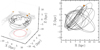 |
Fig. 4 Orbit of Pfleiderer 2 integrated backwards in time for 2.5 Gyr using ORBIT (De Leo et al. 2026a) and accounting for the presence of the bar of the MW. The current position of the cluster is shown with an orange point. The red circle shown in the X-Y projection of the orbit indicates the co-rotational radius, which is equal to 5.79 kpc for the assumed potenital in ORBIT. |
4.4 RLGC2
RLGC2 is a metal-poor cluster located in the thick disc of the MW (Ryu & Lee 2018). Since the available photometry was not deep enough to observe the main sequence and/or sub-giant branch regions, its metallicity has been previously derived via isochrone fitting by fixing its age to the average value of that of metal-poor clusters in the MW (VandenBerg et al. 2013).
As for Pfeiderer 2, all stars in RLGC2 in our sample have compatible spectroscopic Vlos and [Fe/H], yielding average values of Vsys = −313 ± 6 km s−1 and [Fe/H] = −2.33 ± 0.13 dex, which is ~−0.2 dex more metal poor than previous photometric estimates (Ryu & Lee 2018). We find that RLGC2 becomes consistent with the hypothesis of being previously associated with the GSE dwarf galaxy, since it moves on a retrograde and highly eccentric orbit (ecc ~ 0.7) and is therefore only currently crossing the MW thick disc. This result agrees with previous classifications by Massari et al. (2019, eDR3 edition), Libralato et al. (2026), and Callingham et al. (2022), with the latter study also considering a tentative association (p ~ 10%) with the ‘low-energy’–Kraken–Heracles progenitor (LKH, Massari et al. 2019; Kruijssen et al. 2020; Horta et al. 2021; Massari et al. 2026). However, based on our orbital analysis, the cluster orbital energy appears too high and the orbit too retrograde to support such a connection.
5 Summary and conclusion
In this paper, we analysed low-resolution spectroscopic data obtained with MODS@LBT to derive the systemic heliocentric radial velocities and the metallicity for a set of faint and/or highly extinct stellar clusters targeted by the MGCS, whose high-resolution spectroscopic investigation remains challenging with current facilities. For three systems, i.e. Koposov 1, Koposov 2, and Muñoz 1, we validated our measurements against existing spectroscopic determinations available in the literature (Muñoz et al. 2012; Geha et al. 2026) and consistently find excellent agreement. In addition, we present results for Pfleiderer 2 and RLGC2, providing their systemic velocities and spectroscopic metallicity for the first time. We find that Pfleiderer 2 has a Vsys = 6 ± 5 km s−1 and [Fe/H] = −0.75 ± 0.09 dex, while RLGC2 has Vsys = −313 ± 6 km s−1 and [Fe/H] = −2.33 ± 0.13 dex.
For four of the clusters, these new measurements have enabled the first accurate orbital analysis aimed at constraining their origin. We find that one cluster is likely dynamically associated with the Sagittarius dwarf spheroidal galaxy (Koposov 1), one is possibly linked to the Gaia–Sausage–Enceladus merger (RLGC2), one is consistent with an in-situ origin moving on a resonant orbit (Pfleiderer 2), and one remains ungrouped (Koposov 2). Finally, we confirm previous findings that Muñoz 1 occupies a similar region of the integrals of motion space as other clusters associated with the Sag dSph (e.g. Callingham et al. 2022). Nevertheless, it is important to stress that dynamical information alone can sometimes be misleading as orbital parameters alone might not always accurately trace the origin of GCs (see e.g. Pfeffer et al. 2020; Pagnini et al. 2023; Ceccarelli et al. 2025). A definitive assessment of the nature and origin of these systems ultimately requires the combination of dynamics with detailed chemical abundances and precise age determinations.
In recent years, the community has started an extraordinary effort towards a comprehensive census of the MW GC system, especially focusing on observationally challenging clusters. On the photometric side, the final opportunities provided by HST before decommissioning are being leveraged through dedicated surveys such as the MGCS (Massari et al. 2025). Parallel efforts are advancing on the chemical front, including studies based either on available data and current facilities (see e.g. Geisler et al. 2021; Pace et al. 2023; Ferraro et al. 2025; Garro et al. 2026), and next generation wide-field spectroscopic surveys, such as MOONS and 4MOST, with programmes specifically designed to study Galactic stellar clusters and dwarf MW satellites (Gonzalez et al. 2020; Lucatello et al. 2023; Skúladóttir et al. 2023). Together, these complementary initiatives promise to complete our understanding of the formation history of the MW by providing a complete and homogeneous characterisation of its stellar cluster populations.
Acknowledgements
Based on data acquired using the Large Binocular Telescope (LBT) through the program IT-2024B-009 (PI E. Ceccarelli). The LBT is an international collaboration among institutions in the United States, Italy, and Germany. LBT Corporation partners are The University of Arizona on behalf of the Arizona university system; Istituto Nazionale di Astrofisica, Italy; LBT Beteiligungsgesellschaft, Germany, representing the Max-Planck Society, the Astrophysical Institute Potsdam, and Heidelberg University; The Ohio State University; and The Research Corporation, on behalf of The University of Notre Dame, University of Minnesota, and University of Virginia. This work has made use of data from the European Space Agency (ESA) mission Gaia https://www.cosmos.esa.int/gaia), processed by the Gaia Data Processing and Analysis Consortium (DPAC, https://www.cosmos.esa.int/web/gaia/dpac/consortium). Funding for the DPAC has been provided by national institutions, in particular the institutions participating in the Gaia Multilateral Agreement. DM acknowledges financial support from PRIN-MIUR-22 “CHRONOS: adjusting the clock(s) to unveil the CHRONO-chemo-dynamical Structure of the Galaxy” (PI: S. Cassisi) granted by the European Union – Next Generation EU. EC, MB, AM, and MDL acknowledge financial support from the project “LEGO – Reconstructing the building blocks of the Galaxy by chemical tagging” (PI: Mucciarelli) granted by the Italian MUR through contract PRIN2022LLP8TK_001. EC, MB, and AM are grateful to A. Gargiulo for her assistance with the reduction of MODS data using SIPGI. EC thanks F. Cusano for his help in preparing MODS masks, and A. Della Croce for assistance with the figures.
References
- Adamo, A., Bradley, L. D., Vanzella, E., et al. 2024, Nature, 632, 513 [NASA ADS] [CrossRef] [Google Scholar]
- Bellazzini, M., Ibata, R., Malhan, K., et al. 2020, A&A, 636, A107 [NASA ADS] [CrossRef] [EDP Sciences] [Google Scholar]
- Belokurov, V., & Kravtsov, A. 2023, MNRAS, 525, 4456 [NASA ADS] [CrossRef] [Google Scholar]
- Belokurov, V., Zucker, D. B., Evans, N. W., et al. 2006, ApJ, 642, L137 [Google Scholar]
- Belokurov, V., Walker, M. G., Evans, N. W., et al. 2010, ApJ, 712, L103 [NASA ADS] [CrossRef] [Google Scholar]
- Belokurov, V., Erkal, D., Evans, N. W., Koposov, S. E., & Deason, A. J. 2018, MNRAS, 478, 611 [Google Scholar]
- Bennett, M., & Bovy, J. 2019, MNRAS, 482, 1417 [NASA ADS] [CrossRef] [Google Scholar]
- Binney, J., & Tremaine, S. 2008, Galactic Dynamics, 2nd edn. (Princeton University Press) [Google Scholar]
- Callingham, T. M., Cautun, M., Deason, A. J., et al. 2022, MNRAS, 513, 4107 [NASA ADS] [CrossRef] [Google Scholar]
- Carrera, R., Gallart, C., Pancino, E., & Zinn, R. 2007, AJ, 134, 1298 [NASA ADS] [CrossRef] [Google Scholar]
- Carrera, R., Pancino, E., Gallart, C., & del Pino, A. 2013, MNRAS, 434, 1681 [NASA ADS] [CrossRef] [Google Scholar]
- Ceccarelli, E., Mucciarelli, A., Massari, D., Bellazzini, M., & Matsuno, T. 2024, A&A, 691, A226 [NASA ADS] [CrossRef] [EDP Sciences] [Google Scholar]
- Ceccarelli, E., Massari, D., Aguado-Agelet, F., et al. 2025, A&A, 704, A256 [NASA ADS] [CrossRef] [EDP Sciences] [Google Scholar]
- Cerny, W., Li, T. S., Pace, A. B., et al. 2026, arXiv e-prints [arXiv:2602.17652] [Google Scholar]
- Chen, Y., & Gnedin, O. Y. 2024, Open J. Astrophys., 7, 23 [NASA ADS] [Google Scholar]
- Claeyssens, A., Adamo, A., Richard, J., et al. 2023, MNRAS, 520, 2180 [NASA ADS] [CrossRef] [Google Scholar]
- Conn, B. C., Jerjen, H., Kim, D., & Schirmer, M. 2018, ApJ, 852, 68 [NASA ADS] [CrossRef] [Google Scholar]
- De Leo, M., Massari, D., Bellazzini, M., et al. 2026a, A&A, 707, A310 [NASA ADS] [CrossRef] [EDP Sciences] [Google Scholar]
- De Leo, M., Zoccali, M., Olivares-Carvajal, J., et al. 2026b, A&A, 706, A130 [NASA ADS] [CrossRef] [EDP Sciences] [Google Scholar]
- Drimmel, R., & Poggio, E. 2018, RNAAS, 2, 210 [NASA ADS] [Google Scholar]
- Edlén, B. 1966, Metrologia, 2, 71 [CrossRef] [Google Scholar]
- Fadely, R., Willman, B., Geha, M., et al. 2011, AJ, 142, 88 [Google Scholar]
- Ferraro, F. R., Chiappino, L., Bartolomei, A., et al. 2025, A&A, 696, A179 [NASA ADS] [CrossRef] [EDP Sciences] [Google Scholar]
- Forbes, D. A., & Bridges, T. 2010, MNRAS, 404, 1203 [NASA ADS] [Google Scholar]
- Gaia Collaboration (Brown, A. G. A., et al.) 2021, A&A, 649, A1 [NASA ADS] [CrossRef] [EDP Sciences] [Google Scholar]
- Gaia Collaboration (Vallenari, A., et al.) 2023, A&A, 674, A1 [NASA ADS] [CrossRef] [EDP Sciences] [Google Scholar]
- Gargiulo, A., Fumana, M., Bisogni, S., et al. 2022, MNRAS, 514, 2902 [NASA ADS] [CrossRef] [Google Scholar]
- Garro, E. R., Minniti, D., Gómez, M., et al. 2020, A&A, 642, L19 [EDP Sciences] [Google Scholar]
- Garro, E. R., Massari, D., Fernández-Trincado, J. G., et al. 2026, A&A, 706, A338 [NASA ADS] [CrossRef] [EDP Sciences] [Google Scholar]
- Geha, M., Pelliccia, D., Prochaska, J. X., et al. 2026, ApJ, 999, 140 [Google Scholar]
- Geisler, D., Villanova, S., O’Connell, J. E., et al. 2021, A&A, 652, A157 [NASA ADS] [CrossRef] [EDP Sciences] [Google Scholar]
- Gonzalez, O. A., Mucciarelli, A., Origlia, L., et al. 2020, The Messenger, 180, 18 [NASA ADS] [Google Scholar]
- Gran, F., Zoccali, M., Saviane, I., et al. 2022, MNRAS, 509, 4962 [Google Scholar]
- GRAVITY Collaboration (Abuter, R., et al.) 2018, A&A, 615, L15 [NASA ADS] [CrossRef] [EDP Sciences] [Google Scholar]
- Hanuschik, R. W. 2003, A&A, 407, 1157 [NASA ADS] [CrossRef] [EDP Sciences] [Google Scholar]
- Harris, W. E. 2010, arXiv e-prints [arXiv:1012.3224] [Google Scholar]
- Hayes, C. R., Majewski, S. R., Hasselquist, S., et al. 2020, ApJ, 889, 63 [Google Scholar]
- Helmi, A., Babusiaux, C., Koppelman, H. H., et al. 2018, Nature, 563, 85 [Google Scholar]
- Hidalgo, S. L., Pietrinferni, A., Cassisi, S., et al. 2018, ApJ, 856, 125 [Google Scholar]
- Horta, D., Schiavon, R. P., Mackereth, J. T., et al. 2020, MNRAS, 493, 3363 [NASA ADS] [CrossRef] [Google Scholar]
- Horta, D., Schiavon, R. P., Mackereth, J. T., et al. 2021, MNRAS, 500, 1385 [Google Scholar]
- Ibata, R. A., Gilmore, G., & Irwin, M. J. 1994, Nature, 370, 194 [Google Scholar]
- Kim, D., Jerjen, H., Mackey, D., Da Costa, G. S., & Milone, A. P. 2016, ApJ, 820, 119 [Google Scholar]
- Koposov, S., de Jong, J. T. A., Belokurov, V., et al. 2007, ApJ, 669, 337 [Google Scholar]
- Koposov, S. E., Belokurov, V., & Torrealba, G. 2017, MNRAS, 470, 2702 [NASA ADS] [CrossRef] [Google Scholar]
- Kruijssen, J. M. D., Pfeffer, J. L., Chevance, M., et al. 2020, MNRAS, 498, 2472 [NASA ADS] [CrossRef] [Google Scholar]
- Kurucz, R. L. 2005, Mem. Soc. Astron. Ital. Suppl., 8, 14 [Google Scholar]
- Laevens, B. P. M., Martin, N. F., Bernard, E. J., et al. 2015, ApJ, 813, 44 [NASA ADS] [CrossRef] [Google Scholar]
- Libralato, M., Bellini, A., Massari, D., et al. 2026, A&A, 709, A140 [NASA ADS] [CrossRef] [EDP Sciences] [Google Scholar]
- Lucatello, S., Bragaglia, A., Vallenari, A., et al. 2023, The Messenger, 190, 13 [NASA ADS] [Google Scholar]
- Martin, N. F., Venn, K. A., Aguado, D. S., et al. 2022, Nature, 601, 45 [NASA ADS] [CrossRef] [Google Scholar]
- Massari, D. 2025, RNAAS, 9, 64 [Google Scholar]
- Massari, D., Koppelman, H. H., & Helmi, A. 2019, A&A, 630, L4 [NASA ADS] [CrossRef] [EDP Sciences] [Google Scholar]
- Massari, D., Bellazzini, M., Libralato, M., et al. 2025, A&A, 698, A197 [NASA ADS] [CrossRef] [EDP Sciences] [Google Scholar]
- Massari, D., Zerbinati, C., Fanelli, C., et al. 2026, arXiv e-prints [arXiv:2601.18896] [Google Scholar]
- Mau, S., Cerny, W., Pace, A. B., et al. 2020, ApJ, 890, 136 [NASA ADS] [CrossRef] [Google Scholar]
- McMillan, P. J. 2017, MNRAS, 465, 76 [NASA ADS] [CrossRef] [Google Scholar]
- Minelli, A., Bellazzini, M., Mucciarelli, A., et al. 2023, A&A, 669, A54 [NASA ADS] [CrossRef] [EDP Sciences] [Google Scholar]
- Minniti, D., Hempel, M., Toledo, I., et al. 2011, A&A, 527, A81 [NASA ADS] [CrossRef] [EDP Sciences] [Google Scholar]
- Monty, S., Belokurov, V., Sanders, J. L., et al. 2024, MNRAS, 533, 2420 [NASA ADS] [CrossRef] [Google Scholar]
- Moreno, E., Pichardo, B., & Schuster, W. J. 2015, MNRAS, 451, 705 [NASA ADS] [CrossRef] [Google Scholar]
- Moreno, E., Fernández-Trincado, J. G., Schuster, W. J., Pérez-Villegas, A., & Chaves-Velasquez, L. 2021, MNRAS, 506, 4687 [CrossRef] [Google Scholar]
- Muñoz, R. R., Geha, M., Côté, P., et al. 2012, ApJ, 753, L15 [CrossRef] [Google Scholar]
- Muñoz, R. R., Côté, P., Santana, F. A., et al. 2018, ApJ, 860, 66 [CrossRef] [Google Scholar]
- Mucciarelli, A., Bellazzini, M., Ibata, R., et al. 2017, A&A, 605, A46 [NASA ADS] [CrossRef] [EDP Sciences] [Google Scholar]
- Mucciarelli, A., Bellazzini, M., & Massari, D. 2021, A&A, 653, A90 [NASA ADS] [CrossRef] [EDP Sciences] [Google Scholar]
- Mucciarelli, A., Bonifacio, P., & Lardo, C. 2026, A&A, 705, A134 [NASA ADS] [CrossRef] [EDP Sciences] [Google Scholar]
- Navabi, M., Carrera, R., Noël, N. E. D., et al. 2026, MNRAS, 546, stag019 [Google Scholar]
- Newberg, H. J., Yanny, B., & Willett, B. A. 2009, ApJ, 700, L61 [NASA ADS] [CrossRef] [Google Scholar]
- Ortolani, S., Bonatto, C., Bica, E., & Barbuy, B. 2009, AJ, 138, 889 [Google Scholar]
- Pace, A. B., Koposov, S. E., Walker, M. G., et al. 2023, MNRAS, 526, 1075 [CrossRef] [Google Scholar]
- Pagnini, G., Di Matteo, P., Khoperskov, S., et al. 2023, A&A, 673, A86 [NASA ADS] [CrossRef] [EDP Sciences] [Google Scholar]
- Paust, N., Wilson, D., & van Belle, G. 2014, AJ, 148, 19 [Google Scholar]
- Pfeffer, J. L., Trujillo-Gomez, S., Kruijssen, J. M. D., et al. 2020, MNRAS, 499, 4863 [CrossRef] [Google Scholar]
- Pietrinferni, A., Hidalgo, S., Cassisi, S., et al. 2021, ApJ, 908, 102 [NASA ADS] [CrossRef] [Google Scholar]
- Pogge, R. W., Atwood, B., Brewer, D. F., et al. 2010, SPIE Conf. Ser., 7735, 77350A [Google Scholar]
- Portail, M., Wegg, C., & Gerhard, O. 2015, MNRAS, 450, L66 [NASA ADS] [CrossRef] [Google Scholar]
- Queiroz, A. B. A., Chiappini, C., Perez-Villegas, A., et al. 2021, A&A, 656, A156 [NASA ADS] [CrossRef] [EDP Sciences] [Google Scholar]
- Riello, M., De Angeli, F., Evans, D. W., et al. 2021, A&A, 649, A3 [NASA ADS] [CrossRef] [EDP Sciences] [Google Scholar]
- Robin, A. C., Reylé, C., Derrière, S., & Picaud, S. 2003, A&A, 409, 523 [NASA ADS] [CrossRef] [EDP Sciences] [Google Scholar]
- Ryu, J., & Lee, M. G. 2018, ApJ, 863, L38 [NASA ADS] [CrossRef] [Google Scholar]
- Schiavon, R. P., Zamora, O., Carrera, R., et al. 2017, MNRAS, 465, 501 [Google Scholar]
- Searle, L., & Zinn, R. 1978, ApJ, 225, 357 [Google Scholar]
- Sitnova, T. M., Yuan, Z., Matsuno, T., et al. 2024, A&A, 690, A331 [NASA ADS] [CrossRef] [EDP Sciences] [Google Scholar]
- Skúladóttir, Á., Puls, A. A., Amarsi, A. M., et al. 2023, The Messenger, 190, 19 [Google Scholar]
- Starkenburg, E., Hill, V., Tolstoy, E., et al. 2010, A&A, 513, A34 [CrossRef] [EDP Sciences] [Google Scholar]
- Taylor, E. D., Read, J. I., Orkney, M. D. A., et al. 2025, Nature, 645, 327 [Google Scholar]
- Tonry, J., & Davis, M. 1979, AJ, 84, 1511 [Google Scholar]
- VandenBerg, D. A., Brogaard, K., Leaman, R., & Casagrande, L. 2013, ApJ, 775, 134 [Google Scholar]
- Vanzella, E., Calura, F., Meneghetti, M., et al. 2017, MNRAS, 467, 4304 [Google Scholar]
- Vasiliev, E. 2019, MNRAS, 482, 1525 [Google Scholar]
- Vasiliev, E., & Baumgardt, H. 2021, MNRAS, 505, 5978 [NASA ADS] [CrossRef] [Google Scholar]
- Vasiliev, E., Belokurov, V., & Erkal, D. 2021, MNRAS, 501, 2279 [NASA ADS] [CrossRef] [Google Scholar]
- Webb, J. J., & Carlberg, R. G. 2021, MNRAS, 502, 4547 [CrossRef] [Google Scholar]
IRAF was distributed by the National Optical Astronomy Observatory (NOAO), which was managed by the Association of Universities for Research in Astronomy (AURA) under a cooperative agreement with the National Science Foundation.
As such measurements were previously unavailable for all of our targets except Muñoz 1, previous works inferred their orbital properties by adopting a flat prior on the Vsys (e.g. Callingham et al. 2022).
See Massari (2025) for details.
Appendix A Targets information, additional CMDs and spectra
In Table A.1, we report the observational information for targeted stars. In Figs. A.1 - A.2, we present the Gaia CMDs of proper motion selected members of Koposov 1, Koposov 2, A.1 Muñoz 1, and RLGC2 (p > 80%, Vasiliev & Baumgardt 2021). Also, we plot a portion of two stellar spectra per cluster, close to the Hα and CaT lines.
Information on the observations for target stars.
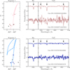 |
Fig. A.1 Same as Fig. 1, but for Koposov 1 (pink) and Koposov 2 (blue). Reference BaSTI isochrone are 7 and 13.5 Gyr old, [Fe/H] = −1.2 dex and [Fe/H] = −2.9 dex, respectively, and α-enanched ([α/Fe] = +0.4 dex). We plot them assuming reddening from Paust et al. (2014) for both clusters, and distances from Paust et al. (2014) and Cerny et al. (2026) for Koposov 1 and Koposov 2. Stars in our sample identified as outliers in Vlos are marked with a coloured cross, if present. |
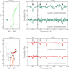 |
Fig. A.2 Same as Fig. 1, but Muñoz 1 (green) and RLGC2 (red). Reference BaSTI isochrone are 12 Gyr, [Fe/H] = −1.4 dex and [Fe/H] = −2.3 dex, respectively, and α-enanched ([α/Fe] = +0.4 dex), assuming distance and reddening from (Muñoz et al. 2012; Ryu & Lee 2018). Stars in our sample identified as outliers in Vlos are marked with a coloured cross, if present. |
Appendix B Output of the BGM model
In Fig. B.1 - B.2, we present the additional output of the BGM model for Koposov 1, Koposov 2, Muñoz 1, and RLGC2. We note that for the first three clusters the spatial window around each cluster center was expanded to 2° to enhance the statistics of the simulated field populations. As the metallicity is available for only one star in Koposov 1, Koposov 2, and Muñoz 1, the BGM metallicity distribution is compared with the measured value and its 1σ uncertainty.
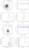 |
Fig. B.1 Same as Fig. 2 for Koposov 1 and Koposov 2. The histogram bin containing the velocity outlier is highlighted with diagonal hatching. For the clusters for which the metallicity is measured for a single star, we plot the corresponding value, and the shaded area represents the associated 1σ uncertainty. |
Appendix C The impact of different distance estimates on the chemodynamical analysis
In Section 3, we adopted a set of homogeneous distance estimates by Paust et al. (2014) for Koposov 1 and Koposov 2, namely 34.9 ± 1.6 kpc and 33.3 ± 1.5 kpc, respectively. However, the literature reports significantly discrepant values for these two systems: in the discovery paper by Koposov et al. (2007), distances of ~ 50 kpc for Koposov 1 and ~ 40 kpc for Koposov 2 were estimated, while more recent works suggest 48.3 kpc for Koposov 1 (Muñoz et al. 2018) and 24 kpc for Koposov 2 (Geha et al. 2026).
Here we briefly assess how adopting these alternative distances affects both the dynamical properties of the clusters and the inferred metallicities. If Koposov 1 is placed at 48.3 kpc, it would become dynamically compatible with an association with the Cetus progenitor, as proposed by Massari et al. (2019, eDR3 edition), and the derived metallicity becomes ~ 0.2 dex more metal-poor. Koposov 2, on the other hand, remains high energy and unassociated for all the distances considered, although larger assumed distances naturally move it at higher orbital energies, Lz, and L⊥. We note that adopting a distance of 24 kpc would make its RGB star ~ 0.15 dex more metal-rich.
Appendix D Comparison with different CaT metallicity relations
To verify and assess the robustness of our results, as well as their sensitivity to the choice of calibration relations, we also derived stellar metallicities using three additional calibration relations. In Table D.1, we report the different metallicity values obtained applying the relations from Carrera et al. (2007), Starkenburg et al. (2010) and Carrera et al. (2013). Given that such relations depends on MV, we computed magnitudes the V band starting from Gaia DR3 photometry (Gaia Collaboration 2023) and using the empiric transformations from Riello et al. (2021). To place all estimates on an homogeneous scale, we also apply the Navabi et al. (2026) calibrations using the MV absolute magnitude.
We do not detect any significant systematic offset between the metallicity obtained with the MG and MV calibrations presented by Navabi et al. (2026), with the only notable exception being RLGC2, for which the metallicity derived using the V-band magnitude is approximately 0.2 dex higher.
More generally, the Navabi et al. (2026) relations tend to yield, on average, slightly more metal-poor metallicities for all stars in our sample, with offsets of ~0.1–0.3 dex relative to the other three adopted calibrations. This is particularly evident for Pfleiderer 2, which is systematically more metal-poor when adopting the Navabi et al. (2026) calibration. The differences reach up to ~ 0.3 dex, being inconsistent at > 2.2σ compared to the other three estimates, which instead provide compatible values. Such inconsistencies are expected in the high metallicity regime (down to [Fe/H] ~ −1.5 dex) and likely reflect the different zero-points of the calibrations. In particular, these relations are anchored at the metal-rich end using the open cluster NGC 6791; however Navabi et al. (2026) adopt a more recent spectroscopic determination of its metallicity, which is lower than the value assumed in earlier works (Carrera et al. 2007, 2013). This naturally shifts the calibration toward slightly more metal-poor values, especially at the metallicity of Pfleiderer 2.
In the end, we find that the Carrera et al. (2007) calibration provides a metallicity that is ~ 0.6 dex more metal-rich for Koposov 2, while the other three relations provide metallicities that are consistent within the uncertainties. This is possibly due to the fact that Koposov 2 lies in a metallicity regime more metal-poor than the range over which the Carrera et al. (2007) relation is well constrained (i.e. down to [Fe/H] ~ −2.2 dex).
Metallicity obtained using different scaling relations and MV as a proxy for the luminosity.
All Tables
Five-dimensional phase-space information (position, proper motion, and distance) from the literature for the target clusters.
Orbital parameters for the observed clusters obtained in a McMillan (2017) potential for the MW.
Metallicity obtained using different scaling relations and MV as a proxy for the luminosity.
All Figures
|
Fig. 1 Left panel: Gaia CMD for Pfleiderer 2 from Vasiliev & Baumgardt (2021). Typical photometric errors at these magnitudes can be found in Gaia Collaboration (2021). All stars with a probability of membership >80% are shown in black, while our selected target stars are plotted in orange. A BaSTI isochrone (Hidalgo et al. 2018, 10 Gyr, [Fe/H] = −0.7 dex, solar-scaled [α/Fe]) is also plotted for reference, taking distance and reddening estimates from Ortolani et al. (2009). Right panel: MODS spectra for the highest and lowest S/N stars among our sample, shown around the Hα and CaT regions (the positions of such absorption lines are indicated with arrows). The same plots for other clusters can be found in Appendix A (see Figs. A.1–A.2). |
| In the text | |
|
Fig. 2 Top row: vector-point diagram (left) for a synthetic Galactic field population (located within 1° from Pfleiderer 2 and selected in the same CMD region populated by the RGB of the cluster) computed with a BGM (Robin et al. 2003). The proper motion of Pfleiderer 2 from Vasiliev & Baumgardt (2021) is indicated with a ‘plus’ marker. On the right panel we display the Vlos distribution of cluster (orange) and field stars from the BGM (grey) as a function of the distance from the cluster centre. Here, stars identified as outliers in Vlos are marked with crosses. Bottom row: heliocentric radial velocity (left) and metallicity (right) distributions for Pfleiderer 2 (orange) and for the BGM synthetic field population (grey). |
| In the text | |
|
Fig. 3 Distribution in the integral-of-motions (E, Lz, L⊥) space of the stellar clusters studied in this paper, compared to all MW GCs (grey points) from Massari et al. (2019, eDR3 edition). As reference, we plot the 1σ ellipses of the distributions of GCs dynamically associated with GSE and Sag dSph, while in-situ GCs are plotted in black. Error bars represent statistical uncertainties from the orbit integration. |
| In the text | |
|
Fig. 4 Orbit of Pfleiderer 2 integrated backwards in time for 2.5 Gyr using ORBIT (De Leo et al. 2026a) and accounting for the presence of the bar of the MW. The current position of the cluster is shown with an orange point. The red circle shown in the X-Y projection of the orbit indicates the co-rotational radius, which is equal to 5.79 kpc for the assumed potenital in ORBIT. |
| In the text | |
|
Fig. A.1 Same as Fig. 1, but for Koposov 1 (pink) and Koposov 2 (blue). Reference BaSTI isochrone are 7 and 13.5 Gyr old, [Fe/H] = −1.2 dex and [Fe/H] = −2.9 dex, respectively, and α-enanched ([α/Fe] = +0.4 dex). We plot them assuming reddening from Paust et al. (2014) for both clusters, and distances from Paust et al. (2014) and Cerny et al. (2026) for Koposov 1 and Koposov 2. Stars in our sample identified as outliers in Vlos are marked with a coloured cross, if present. |
| In the text | |
|
Fig. A.2 Same as Fig. 1, but Muñoz 1 (green) and RLGC2 (red). Reference BaSTI isochrone are 12 Gyr, [Fe/H] = −1.4 dex and [Fe/H] = −2.3 dex, respectively, and α-enanched ([α/Fe] = +0.4 dex), assuming distance and reddening from (Muñoz et al. 2012; Ryu & Lee 2018). Stars in our sample identified as outliers in Vlos are marked with a coloured cross, if present. |
| In the text | |
|
Fig. B.1 Same as Fig. 2 for Koposov 1 and Koposov 2. The histogram bin containing the velocity outlier is highlighted with diagonal hatching. For the clusters for which the metallicity is measured for a single star, we plot the corresponding value, and the shaded area represents the associated 1σ uncertainty. |
| In the text | |
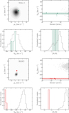 |
Fig. B.2 Same as Fig. B.1 for Muñoz 1 and RLGC2. |
| In the text | |
Current usage metrics show cumulative count of Article Views (full-text article views including HTML views, PDF and ePub downloads, according to the available data) and Abstracts Views on Vision4Press platform.
Data correspond to usage on the plateform after 2015. The current usage metrics is available 48-96 hours after online publication and is updated daily on week days.
Initial download of the metrics may take a while.