


| Issue |
A&A
Volume 711, July 2026
|
|
|---|---|---|
| Article Number | A155 | |
| Number of page(s) | 11 | |
| Section | Stellar atmospheres | |
| DOI | https://doi.org/10.1051/0004-6361/202659578 | |
| Published online | 17 July 2026 | |
Ag I model atom and the 3D non-LTE solar silver abundance
1
Theoretical Astrophysics, Department of Physics and Astronomy, Uppsala University,
Box 516,
751 20
Uppsala,
Sweden
2
Department of Materials Science and Applied Mathematics, Malmö University,
205 06,
Malmö,
Sweden
3
Centre Spatial de Liège, Université de Liège,
avenue Pré Aily,
4031
Angleur-Liège,
Belgium
4
Space sciences, Technologies and Astrophysics Research (STAR) Institute, Université de Liège,
Allée du 6 août, 17, B5C,
4000
Liège,
Belgium
5
Atomic, Molecular and Optical Physics Division, Physical Research Laboratory, Navrangpura,
Ahmedabad
380009,
India
★ Corresponding author: This email address is being protected from spambots. You need JavaScript enabled to view it.
Received:
23
February
2026
Accepted:
29
April
2026
Abstract
Silver is an important light neutron-capture element whose stellar abundances can help constrain the origin of the weak r-process. The Sun is an important reference point for such studies; moreover, being a moderately volatile element in CI chondrites, the solar silver abundance is interesting as a diagnostic for the debated Sun-CI abundance versus condensation temperature trend. These studies require accurate silver abundances that go beyond the commonly used assumptions of one-dimensional (1D) atmospheres and local thermodynamic equilibrium (LTE); however, no consistent 3D non-LTE analysis of silver has been available to date. We present a new Ag I model atom built from carefully curated radiative and collisional data, including newly computed oscillator strengths using an ab initio multi-configurational Hartree-Fock method and inelastic hydrogen collision rates based on a combined asymptotic and free-electron-model approach. We assessed modelling uncertainties via targeted sensitivity tests, finding the results to be most sensitive to the hydrogen-collision data. Applying the model to the solar Ag I 328 and 338 nm resonance lines, we find severe positive-abundance corrections from coupled 3D and non-LTE effects. Using revised equivalent-width measurements, we derive a recommended solar 3D non-LTE silver abundance of log εAg = 1.15 ± 0.08. This is an increase of 0.19dex relative to the current reference value. Our ab initio model significantly reduces the discrepancy with the meteoritic value from 0.25 to 0.06 dex; moreover, this residual offset is consistent with what was recently reported for other moderately volatile elements. The Sun provides the benchmark test for the first silver non-LTE model atom presented here. In subsequent work, this model will be applied to determine 3D non-LTE silver abundances in metal-poor dwarfs and giants, enabling improved constraints on Galactic chemical evolution and weak r-process nucleosynthesis.
Key words: atomic processes / line: formation / radiative transfer / Sun: abundances / Sun: photosphere
© The Authors 2026
 Open Access article, published by EDP Sciences, under the terms of the Creative Commons Attribution License (https://creativecommons.org/licenses/by/4.0), which permits unrestricted use, distribution, and reproduction in any medium, provided the original work is properly cited.
This article is published in open access under the Subscribe to Open model. This email address is being protected from spambots. You need JavaScript enabled to view it. to support open access publication.
1 Introduction
Silver is a light neutron-capture element (Z=47) whose astrophysical origin, and the relative yields of its different production processes and sites, have long been of interest. Yet, stellar constraints on silver remain sparse, as only two Ag I resonance lines are observable, and both lie in the near-UV, where they are strongly affected by blends. Hansen & Primas (2011) and Hansen et al. (2012) are recognised as the first works in which the silver abundance was analysed for a large sample of stars. Even before these papers, several studies (e.g. Honda et al. 2006; François et al. 2007; Sneden et al. 2008; Roederer et al. 2010) found that lighter r-process elements (i.e. 34 ≤ Z < 56) exhibit a departure from the predicted Solar System r-process residual pattern compared to the heavier r-process elements showing a universal r-process distribution. This suggests that more than one r-process channel contributes; they are commonly referred to as a ‘weak’ and a main channel (e.g. Wanajo & Ishimaru 2006; Ott & Kratz 2008; Kratz et al. 2007; Montes et al. 2007; Farouqi et al. 2009).
Silver can be considered a tracer of the weak r process. First, it is produced predominantly by the r process; Goriely (1999), Sneden et al. (2008), and Prantzos et al. (2020) predicted that nearly 80% of Solar-System silver originates from r-process nucleosynthesis. Moreover, silver lies near the middle of the atomic-number range where the lighter r-process elements deviate from the main solar-scaled r-process distribution, making it well placed to probe any ‘weak’ component. In their paper, Hansen et al. (2012) supported this interpretation by showing a strong anti-correlation at low metallicities between silver and europium (formed by the main r-process). Their findings were later confirmed by Wu et al. (2015), which increased the sample of stars with observed silver abundances to solar and super-solar metallicities, and more recently by Huang et al. (2025), which extended it to extremely metal-poor stars. However, these studies all report large star-to-star scatter in the silver trends, and Hansen & Primas (2011) additionally found an abundance difference of around 0.5 dex between dwarfs and giants at similar metallicity.
Silver in our Solar System also exhibits a puzzling discrepancy. The currently adopted solar photospheric value is that of Grevesse et al. (2015), log εAg = 0.96 ± 0.101, which was derived by synthesising the two Ag I UV resonance lines using a threedimensional (3D) radiation-hydrodynamical model atmosphere. However, as discussed in Asplund et al. (2021), the presentday solar photospheric abundance of silver differs greatly from that inferred from CI chondrites, with the value of Grevesse et al. (2015) being 0.25 dex lower than the meteoritic value from Lodders (2021).
All of the aforementioned studies have derived silver abundances under the assumption of local thermodynamic equilibrium (LTE), be it in 1D for large samples of stars (e.g. Hansen & Primas 2011; Hansen et al. 2012; Wu et al. 2015; Huang et al. 2025), or in 3D for the Sun (Grevesse et al. 2015). Thus, the potential impact of 3D non-LTE effects on the star-to-star scatter and the dwarf-giant offset in metal-poor stars, as well as on the inconsistency between the solar photospheric silver abundance and that found in primitive meteorites, has not yet been assessed. Detailed 3D non-LTE modelling is therefore needed to clarify the formation channels of silver and its role as a weak r-process tracer, as well as the true solar reference abundance.
To this day, there are no non-LTE calculations of silver in the literature, likely in part because of incomplete atomic data for silver. Non-LTE modelling requires a so-called model atom containing extensive radiative and collisional data. In this paper, we compile the best available atomic data for silver that are needed for non-LTE spectrum synthesis and compute missing ingredients where necessary, such as for the inelastic collisions with neutral hydrogen (Sect. 2). We investigated the 3D and non-LTE effects on the formation of the Ag I 328 and 338 nm resonance lines in the solar photosphere (Sect. 3). We calculated the 3D non-LTE abundance correction for the Sun and re-evaluated the solar silver abundance in comparison with previous determinations (Sect. 4). Our goal is to benchmark the model atom on the Sun, prior to calculating and applying 3D non-LTE abundance corrections to other late-type stars, which will be addressed in future work (Sect. 5).
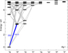 |
Fig. 1 Grotrian diagrams for Ag I illustrating the model atom. The transitions highlighted in blue correspond to the two Ag I diagnostic lines analysed in this work (vacuum wavelengths). The horizontal dotted line marks the silver ionisation limit. |
2 Methods
2.1 Model atom
A model atom for the non-LTE modelling of Ag I was constructed for this study. The structure of the model is illustrated in Fig. 1. We present an overview of the different ingredients used in the model here.
The model consists of 57 energy levels with fine structure taken from the NIST database (Kramida et al. 2022). This includes five fine-structure levels of Ag II, namely the ground state, as well as the first two excited terms. For the bound-bound radiative transitions, only seven oscillator strengths (f values) can be found on NIST.
These seven oscillator strengths from NIST were then complemented with values for 53 more transitions via ab initio combined, multi-configurational, Dirac-Hartree-Fock, and relativistic configuration interaction (MCDHF+RCI) calculations performed using the GRASPG package (Si et al. 2025), which is an extension of GRASP (Froese Fischer et al. 2019), for the important low-lying levels up to 4d108s2S1/2 (6.89 eV). Further details about the methods and results of this calculation can be found in Jönsson et al. (2026). In the paper, the computed excitation energies and transition rates were compared to results from Fockspace multi-reference coupled cluster (FSMRCC) calculations (e.g. Sahoo et al. 2025), and a good agreement was generally found. Moreover, the MCDHF+RCI lifetimes were in agreement with experimental lifetimes.
For the two diagnostic lines, we adopted the oscillator strengths from NIST, with log gf = −0.046 and log gf = −0.356 for the 328 and 338 nm line, respectively. These values agree with the experimental values of log gf = −0.021 and −0.333 from Carlsson et al. (1990). They are also in close agreement with the calculated MCDHF+RCI (log gf = −0.036 and log gf = −0.352) and FSMRCC (log gf = −0.003 and log gf = −0.315) values.
For the transitions including higher levels, oscillator strengths were taken from Civiš et al. (2010), calculated using the Fues-model-potential (FMP) approach. A comparison between the two sets of oscillator strengths and their impact on the non-LTE abundance can be found in Sect. 4.1.
Natural broadening coefficients were calculated via

where Aul′ and All′ are transition rates from the upper and lower level of the ul transition, respectively, to all other lower levels (e.g. Gray 2022). Pressure broadenings due to hydrogen collisions were obtained by interpolating the tables of Anstee, Barklem, and O’Mara (ABO theory; Barklem et al. 2000) when available, and the classical Unsöld theory was applied otherwise, adopting a fudge factor of 2.0 (see the discussion in Barklem 2016a). In addition, hyperfine structure and isotopic contributions were added for the two diagnostic lines. The same values were adopted as in Hansen et al. (2012), where the authors derived new hyperfine components, instead of using those from Ross & Aller (1972) as is commonly done in abundance studies of the Ag I resonance lines in the literature (e.g. Wu et al. 2015; Huang et al. 2025); this is because they only included two hyperfine components per isotope, missing one component. The adopted isotopic ratio is 51.84% for isotope 107 and 48.16% for isotope 109 (Asplund et al. 2021). Nevertheless, we found that the hyperfine and isotopic splitting only affects the non-LTE equivalent widths of the two diagnostic lines by around 0.01 dex in the solar photosphere.
Photoionisation cross-sections were estimated under the hydrogenic approximation using the Kramers formula (e.g. Rutten 2003):

in units of cm2, where neff is the effective principal quantum number and ν is the frequency. The Gaunt factor was set to unity.
The rate coefficients for excitation via electron collisions were calculated using the recipe of Seaton (1962) for the transitions with available transition rates, A. For the other lines, the semi-empirical van Regemorter recipe (van Regemorter 1962) was used (assuming an effective oscillator strength of 0.001/gl, with gl the statistical weight of the lower level) to estimate the Einstein coefficients for spontaneous emission entering the recipe. For ionisation via electron collisions, the empirical formula given in Allen (1973) was adopted.
Finally, for excitation and charge transfer via neutral hydrogen collisions, we performed calculations based on the asymptotic model approach described in Barklem (2016b, 2017a) for the rate coefficients, for all the energy levels included in the model atom (except h states). For the parentage coefficients, appearing in the expression of the wave function for the Ag + H quasi-molecule used to calculate the potentials and couplings, we adopted the same values calculated for Cu I in Caliskan et al. (2025) since they are homologous elements and therefore have very similar energy structures. We combined the asymptotic model rates with excitation-rate coefficients calculated via the code from Barklem (2017b), which is based on the free electron model by Kaulakys (1991), for all Ag I energy levels. It was shown in the literature that the latter approach may better account for the transition mechanisms involving highly excited levels near the relevant ionic limit and for states where the avoided crossing occurs at long and short internuclear distances (e.g. Amarsi et al. 2018a). Combining the two methods therefore prevents us from underestimating the hydrogen collisions. Since these two approaches do not account for fine structure, we redistributed the rate coefficients among fine-structure levels by dividing the coefficients calculated without fine-structure by the total number of final states; we did so following Boltzmann distributions. Finally, we also assigned very large rate coefficients for transitions between fine-structure levels, motivated by the Massey criterion (Massey 1949), which suggests that inelastic collisions efficiently couple these levels referred to as ‘relative LTE’.
As can be seen from the model atom in Fig. 1, the energy levels belonging to the 4d95s5p configuration in the quartet spin system are included in the model atom, but they are not connected by bound-bound radiative transitions in the model. The transitions connecting the quartet system to the 4d10 levels in the doublet system correspond to two-electron transitions and thus are expected to be intrinsically weak, as are the spin-forbidden transitions connecting the quartet system to the 4d95s2 levels in the doublet system. In fact, to our knowledge, there are no oscillator strengths for these transitions available in the literature, likely because the lines are too weak to measure, and because it is challenging to accurately calculate the atomic structure (these levels are known to perturb the energy structure, as discussed for the homologous system Au I in Caliskan et al. 2024). Consequently, in the present model, these transitions couple to the doublet system only via collisional transitions, as well as to the excited levels of Ag II via both collisions and photoionisations. Similarly, the two 2H levels are only connected to the rest of the levels via collisions/photoionisations due to a lack of oscillator strengths for these transitions.
2.2 Model atmospheres
We illustrate the different model solar atmospheres used in this work in the lower panel of Fig. 2. The 3D model atmosphere is the same one as was first described in Amarsi et al. (2018a). In brief, it is a 3D radiation-hydrodynamics simulation that was calculated using the STAGGER code (e.g. Collet et al. 2018; Stein et al. 2024). The model is wide enough to encompass around ten granules at any given time and spans around six pressure scale heights below the optical surface and eight pressure scale heights above it, with a resolution that is comparable to that of the STAGGER-grid (Magic et al. 2013). The parameters of the model are close to the standard solar values (Prša et al. 2016), with the gravitational acceleration corresponding to log g = 4.44 [cm s−2] and a time-averaged effective temperature of Teff = 5773 K with a snapshot-to-snapshot standard deviation of 16 K. The model was computed using the solar elemental abundances of Asplund et al. (2009). In the subsequent post-processing calculations (Sect. 2.3), the silver abundance was allowed to vary freely, under the assumption that it is a trace element with no influence on the background pseudostatic model atmosphere.
In order to obtain differential abundance corrections, we also performed 1D calculations using a 1D version of the 3D STAGGER model, which was calculated using the Atmo code (see Appendix A of Magic et al. 2013). This was constructed using the same equation of state, opacity binning, and solar parameters as for the 3D model.
Finally, we also performed calculations on the temporal and horizontal averages of the 3D model solar atmosphere. Details of its construction can be found in Amarsi et al. (2018a). We refer to this as the mean 3D 〈3D〉 model hereafter. This is useful for decomposing the 3D effect into a granulation effect and a stratification effect (e.g. Lind & Amarsi 2024), as discussed in Sect. 3.2. Moreover, the sensitivity tests in Sect. 4.1 were based on this model rather than on the full 3D model to save computational time.
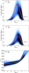 |
Fig. 2 Top and middle : non-LTE contribution functions (CFs) to the line depression in the vertical intensity (e.g. Amarsi 2015) for the two diagnostic Ag I lines as a function of vertical optical depth. The contours show the distributions in the 3D model’s solar atmosphere, and the CF in 1D and (3D) are overplotted. All are normalised to the maximum of the 1D LTE CF of the 328 nm line. Bottom : temperature stratification of the 1D, (3D), and 3D model solar atmospheres. |
Ag I abundances inferred from different spectrum-synthesis models.
2.3 Line-formation calculations and abundance corrections
The statistical equilibrium and synthetic emergent spectra were calculated using the 3D non-LTE radiative-transfer code Balder (Amarsi et al. 2018b), which is a custom version of Multi3D (Botnen & Carlsson 1999; Leenaarts & Carlsson 2009). Using the code Blue (Amarsi et al. 2016; Zhou et al. 2023), the equation-of-state and background continuous opacities were calculated on the fly, whereas background line opacities were pre-computed and interpolated onto the model atmosphere at run time. The non-LTE iterations used 26 rays on the unit sphere based on the Lobatto quadrature for the polar angle and a trapezoidal quadrature for the azimuthal angle (Amarsi et al. 2024). While this study is primarily based on disc-centre intensities, disc-integrated fluxes were also calculated, integrating over 41 rays on the unit hemisphere.
For the 3D model atmosphere, calculations were performed on ten snapshots. As in previous work (e.g. Amarsi et al. 2018a), these were down-sampled by a factor of three in each of the horizontal dimensions and refined in the vertical dimension prior to post-processing with Balder. For the 1D and 〈3D〉 models, microturbulent broadening was introduced and set to 1.0 km s−1. No microturbulent broadening was used for the 3D calculations, as these effects primarily reflect the granulation contrast rather than true turbulent broadening (e.g. Nordlund et al. 1997), and so they are naturally included in the 3D radiative-transfer calculations with Balder.
Emergent spectra were calculated for seven different abundances of silver, from −0.6 dex to +0.6 dex in steps of 0.2dex, without the inclusion of background line opacities. This was also repeated without foreground (silver) line opacities to determine the theoretical continuum and thereby arrive at continuum-normalised spectra. Equivalent widths were determined by direct integration across the normalised and unblended Agl 328 and 338 nm lines.
We used the notation ΔI(3N − 1L) to indicate the 3D non-LTE (3N) versus 1D LTE (1L) abundance correction for the disc-centre intensity (I). The abundances were determined via spline interpolation of the silver abundance as a function of the calculated logarithmic equivalent width onto the input logarithmic equivalent width measured at the solar disc centre (listed in Table 1). We used similar notation for other abundance corrections, for example ΔI(3N – 3L) for the 3D non-LTE versus 3D LTE abundance correction.
3 Results
3.1 Non-LTE effects
To interpret the non-LTE effects, it is useful to look at how they affect the level populations. We illustrate these departures from LTE using the departure coefficients (b ≡ nNLTE/nLTE), which are shown in Fig. 3. The figure includes the first six Ag I levels in order of increasing energy (fine-structure components in relative LTE in our model and therefore having identical departure coefficients, are only plotted once), as well as the highly excited 5s5p4F5/2 level and the ground state of Ag II.
The two diagnostic resonance lines are from transitions between the ground level, 5s2S1/2, and the first and third excited levels, 5p2P1/2,3/2. When we look at level populations in LTE, we can see that the majority species is Ag II, and almost all of the Ag I atoms lie in the ground state. The departure coefficients reflect the fact that in non-LTE, the population of the ground level is depleted by the two resonance lines via excitations, as we can tell from the dip around logτR ≈ −1; corresponding to the region where the lines form (see Fig. 2), while they overpopulate the first and third excited levels, 4d105p2P1/2,3/2. The second and fourth excited levels, 5s2 2D5/2,3/2, show the same pattern for the departure coefficients as the 5p 2P1/2,3/2 throughout the atmosphere, indicating that efficient collisions push these levels towards relative LTE. The more highly excited states in the doublet system are similarly connected via effective collisions and therefore have very similar departure coefficients (compare the departure coefficients of 6p2P1/2 with the 5d 2D3/2). This network of effective collisions propagates the overexcitation from the resonance lines all the way to the Ag II levels, causing an over-ionisation.
The Ag I 328 and 338 nm lines thus drive the non-LTE effects in the system. To further demonstrate this, we carried out a test where the oscillator strengths of both lines were set to zero when calculating the statistical equilibrium. When doing so, the statistical equilibrium shifted much closer to LTE. When subsequently calculating the emergent spectra based on these converged populations, the Ag I 328 and 338 nm lines appeared much deeper, with the difference between LTE and non-LTE equivalent widths being only 0.02 dex in the (3D) model atmosphere.
The departure coefficients of the excited level of 6s 2S1/2 look slightly different from the other excited levels, exhibiting a flatter trend closer to unity. This trend can be explained by a competition between collisional coupling of this level to more excited levels, versus photon losses in the relatively strong AgI 768.8 and 827.5 nm doublet, which connect this level to the 5p 2P1/2,3/2 levels (with log gf = –0.48 and –0.15 in the present model, respectively). Switching this doublet off, the departure coefficients of the 6s 2S1/2 would appear qualitatively similar to those of the more excited levels such as the 6p 2P1/2 and 5d 2D3/2.
Finally, we also show the departure coefficients of the 4d95s5p 4F5/2 level in order to illustrate the case of the 4d95s5p levels where the 4d10 core is excited. As explained in Sect. 2.1, in the model atom the 4d9 levels in the quartet system only couple to the levels in the doublet system via collisions. Efficient coupling exists via electron collisions between the 4d9 quartet levels and the 4d10 levels of similar excitation energies. This competes with efficient coupling via hydrogen collisions between the 4d9 quartet levels and the 4d95 s2 levels in the doublet system. The result of this competition is that the departure coefficients of the 4d9 quartet levels appear in between those of the excited 4d10 levels (which appear similar to those for the 6p 2P1/2 and 5d 2D3/2 in Fig. 3), and those of the 4d95s2 levels in the doublet system.
The abundances inferred from the different spectrum synthesis models are given in Table 1. Based on that, the line-averaged abundance correction, ΔI(1N – 1L), is +0.21 dex. The abundance corrections, here based on measured equivalent widths, are very close for both lines; this can be understood by the fact that they connect the same levels (just different fine structures) and have similar formation depths. Taking non-LTE into account, both diagnostic lines become weaker, which in turn gives a larger non-LTE abundance. The weakening of the lines in non-LTE is the result of the combination of an opacity effect, where the line’s opacity decreases due to the non-LTE population of the lower level becoming smaller than the LTE value (b < 1 in Fig. 3, first panel); and the source function effect, where the line source function increases due to bu /bι > 1 at the depth where the lines form.
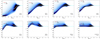 |
Fig. 3 Departure coefficients for seven energy levels of Ag I (in increasing excitation energy from left to right) and the ground level of Ag II. The contours show the distributions in the 3D model’s solar atmosphere. The departure coefficients calculated in the (3D) and 1D models are overplotted. |
3.2 3D effects
The total 3D effect is quantified by ΔI(3N – 1N). To further our understanding, we separate this 3D effect into two components: granulation, (the direct effect) and mean stratification (the indirect effect) (e.g. Lind & Amarsi 2024).
The direct effect can be quantified by the difference between the 3D and (3D) non-LTE abundances, ΔI(3N - 〈3D〉N) since granulation is present in the 3D solar model atmosphere but absent from the (3D) model (e.g. Caffau et al. 2011). We find that the two diagnostic lines exhibit different granulation effects, which we attribute to their different equivalent widths and hence their positions on the curve of growth. In Fig. 6b of Lind & Amarsi (2024), lines that approach the saturated part of the curve of growth show a rapid increase towards more positive ΔI(3N - 〈3D〉N). In our case, the 328 nm line is the stronger of the two, with a reduced equivalent width of –5.0, and yields ΔI(3N - 〈3D〉N) = +0.03 dex, which is consistent with lines of other minority neutral species at similar reduced equivalent widths in Lind & Amarsi (2024). By contrast, the weaker 33 8 nm line, with a reduced equivalent width of –5.2, shows a much smaller correction of +0.01 dex. The line-averaged granulation effect is ΔI(3N - 〈3D〉N) = +0.02 dex. This positive granulation effect may reflect that the adopted microturbulence of ξmic;1D in the (3D) model is too high, overestimating the de-saturation effect of the 3D velocity fields. Meanwhile, the indirect effect can be quantified via the line-averaged ΔI(〈3D〉N - 1N) abundance correction. As the (3D) model has a shallower temperature gradient, the (3D) line profile is weaker than the 1D one, and the abundance difference is always positive, Δ1(〈3D〉N – 1N) = +0.06 dex, again in agreement with the values for minority species in the Sun in the Δstrat versus log10(Wλ/λ) plot from Fig. 6a in Lind & Amarsi (2024). The indirect effect is stronger than the direct effect, thus dominating the overall 3D effect. They both contribute to weakening the 3D non-LTE line, and therefore add up to give a positive line-averaged abundance correction, ΔI(3N – 1N), of +0.07dex.
Finally, we illustrate the synthetic line profiles in Fig. 4. The 3D profiles have broader wings than the 1D and (3D) ones for a fixed ξmic;1D of 1km s−1. One should note that no macroturbulence was added to the 1D and (3D) line profiles, which contributes to the differences relative to the 3D line profile, particularly in the wings. Moreover, the 3D line profiles are slightly blueshifted relative to the 1D and (3D) line profiles and clearly display a C-shape asymmetry. Both of these features are a consequence of integrating the lines over the surface of the 3D model, sampling both the hot, up-flowing granules and cool, down-flowing lanes (e.g. Dravins 1982; Asplund et al. 2000).
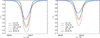 |
Fig. 4 Synthetic line profiles of the diagnostic Ag I lines computed in LTE and non-LTE using different solar model atmospheres. No macroturbulence was added to the lines. |
3.3 Coupling between 3D and non-LTE effects
We discuss the non-LTE and 3D effects individually in Sects. 3.1 and 3.2, but in reality the two can interact. In the literature, it is common to see that the 3D LTE and 1D non-LTE abundance corrections are separately applied to the 1D LTE abundance (see, e.g. Table 1 of Asplund et al. 2021). However, in the case of a coupling between the 3D and non-LTE effects, this procedure can break down, and this approximate ‘3D + non-LTE’ abundance may differ by up to 0.5 dex from the fully consistent 3D non-LTE result, at least in metal-poor stars (Lagae et al. 2023).
To quantify this 3D/non-LTE coupling, we compare the line-averaged ΔI(3N – 3L) and ΔI(1N – 1L) abundance corrections. We find Δ1(3N – 3L) – Δ1(1N – 1L) = 0.07dex, indicating that there is a coupling between the 3D and non-LTE effects for Ag I in the Sun, with the 3D models yielding larger non-LTE corrections.
A plausible explanation is that the steeper temperature gradients within the inhomogeneous 3D radiation-hydrodynamical model atmosphere enhance the non-local radiation field, leading to more photon pumping in the UV resonance lines, analogous to that described for Fe I in 3D models of metal-poor stars (e.g. Amarsi et al. 2016). This scenario is further supported by the positive Δ1(3N – 3L) – ΔI(〈3D〉N – 〈3D〉L) difference (+0.07 dex), showing the enhancement of the non-LTE departures when moving to the full, inhomogeneous 3D model.
Overall, the coupled 3D and non-LTE effects lead to a severe line-averaged abundance correction of Δ1(3N – 1L) = +0.28 dex. We briefly note that our calculated abundance correction is similarly large in the disc-integrated flux (ΔF(3N – 1L) = +0.29 dex). Both the 3D and non-LTE departures act in the same direction on the lines’ equivalent widths, producing positive abundance corrections, but the non-LTE effect is more severe than the 3D effect. We thus find that 1D LTE is the poorest approximation, while 1D non-LTE is closer to the full 3D non-LTE result than 3D LTE.
4 Discussion
4.1 Sensitivity to the radiative and collisional data
In order to estimate the sensitivity of non-LTE abundances to uncertainties in the model atom, we performed several tests by varying the atomic data in the latter. The results of our tests are summarised in Fig. 7, where we show the difference of the equivalent widths in the fiducial model versus the test model for the two AgI diagnostic lines in the (3D) solar model atmosphere for a fixed silver abundance of 0.94 dex. These differences are shown for both lines, although they show similar sensitivities as expected, as they belong to the same fine structure multiplet and are of similar strength.
First, we tested the impact of the newly calculated MCDHF+RCI oscillator strengths by replacing them with the less certain oscillator strengths from Civiš et al. (2010) when possible; this corresponds to ‘log gfFMP’ in Fig. 7. We ended up switching the f values of 40 bound-bound transitions out of 183, with the seven experimental oscillator strengths from NIST remaining unchanged. This had little to no effect on the non-LTE equivalent widths of the Ag I 328 and 338 nm lines. Indeed, when we compare the MCDHF+RCI and FMP oscillator strengths in Fig. 6, we see a quite good agreement for the strongest lines that can have the largest impact on the statistical equilibrium, as also shown in Jönsson et al. (2026). Therefore, switching between these oscillator strengths does not significantly change the abundances inferred from the Ag I 328 and 338 nm lines.
To estimate the impact of the photoionisation cross-sections on the non-LTE solution, it would be useful to compare the hydrogenic approximation with cross-sections obtained using a more sophisticated method. Such a comparison would also provide good grounds to discuss how realistic the widely used hydrogenic approximation is. However, since photoionisation data for Ag I are lacking in the literature, we instead first considered the case of the homologous element Cu I. In Fig. 5, we compare hydrogenic cross-sections with the R-matrix calculations of Liu et al. (2014) for the ground and second excited levels of Cu I. The hydrogenic cross-sections are of the same order as the average R-matrix cross-sections (within a factor of 10), but they typically fail to capture the detailed structure, such as the resonances. Motivated by this comparison, we tested the impact of the approximate hydrogenic cross-sections in Ag I by decreasing and increasing all the cross-sections by a factor of ten. The resulting non-LTE equivalent widths for Ag I 328 and 338 nm vary only marginally, i.e. by 0.005 (for 10 times smaller) to 0.001 dex (for 10 times larger) for both lines. We therefore conclude that these lines are insensitive to large perturbations of the photoionisation data and that a more detailed treatment of these processes seems unnecessary for the present study. This weak sensitivity can be explained by the close collisional coupling of the Ag I excited levels to the Ag II levels, combined with the photon losses caused by the resonance lines, driving the non-LTE effects (as explained in Sect. 3.1) and effectively compensating for the population changes caused by photoionisation.
Next, we tested the impact of collisional rates by decreasing and increasing the different rates by a factor of ten. Figure 7 shows that the collisional charge transfer (i.e. both electron and hydrogen ionisation) has a negligible effect on the equivalent widths compared to collisional excitation, with the biggest impact from the hydrogen ionisation: Δ(EW) of –0.003 dex. A factor of ten increase in the electron-impact collisional excitations also has a negligible impact on the equivalent widths of the diagnostic lines (+0.005 dex).
Finally, as explained in Sect. 2.1, new Ag + H collisional rates were calculated for the first time using the asymptotic and free electron models. We found that a factor of ten increase in the collisional rates has the largest impact on the non-LTE equivalent widths, making the model more sensitive to the hydrogen collision data than to any of the other aforementioned ingredients. Barklem (2016a) argued that the asymptotic methods are accurate to within a factor of ten. If this is a realistic uncertainty for the asymptotic hydrogen collisional cross-sections, we can quantify the corresponding abundance uncertainty. The line-averaged abundance correction, ΔI(〈3D〉N - 〈3D〉L), went from 0.20 dex down to 0.12 dex when the hydrogen collisions were increased and up to 0.22 dex when they were decreased. Taking half the range, we estimate a 0.05 dex contribution to the overall abundance uncertainty.
This difference in the equivalent widths is largely driven by two collisional transitions, 4d 105s 2S1/2 → 4d 105p 2P1/2,3/2, which makes sense given that these are also the transitions behind the diagnostic lines and that they compete directly with the over-excitation effect discussed in Sect. 3.1. The rates for these transitions are zero in the asymptotic model and relatively strong in the free-electron model, highlighting the importance of the latter to avoid missing important collisional transitions (e.g. Amarsi et al. 2018a). We further discuss the reliability on the hydrogen collision data in Sect. 4.3.
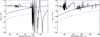 |
Fig. 5 Photoionisation cross-sections for neutral copper from the ground (3d104s; left) and second excited (3d104p; right) states. The black curves show the R-matrix cross-sections from Liu et al. (2014), while the blue curve shows the hydrogenic approximation; the dashed blue curves indicate the hydrogenic cross-sections shifted by ±1 dex. |
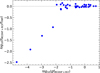 |
Fig. 6 Comparison of newly calculated MCDHF+RCI oscillator strengths, with oscillator strengths from Civiš et al. (2010) based on the FMP approach. |
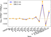 |
Fig. 7 Changes in (3D) non-LTE equivalent widths of the two Ag I diagnostic lines when varying atomic data in the model atom and the background lines (‘test’) compared to the fiduciary model. |
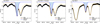 |
Fig. 8 Fits to Liège disc-centre intensity spectrum, with 3D LTE spectrum synthesis and the VALD line list. The shaded black area reflects the uncertainty in placing the continuum. The shaded blue area shows the equivalent width of the pure Ag I line. Left and middle : synthesis of Ag I 328 nm line, omitting and including a predicted Fe I blend, respectively; the recommended equivalent width for this line in Table 1 is based on the mean of these two results. |
4.2 Sensitivity to the background line opacities
The background line opacities were not calculated internally, they were pre-calculated in LTE assuming a solar chemical composition. We cannot ignore the impact of the background lines, especially of those that overlap with the Ag I diagnostic lines, as these drive the non-LTE effects and are heavily affected by background lines.
It is important to assess the sensitivity of the non-LTE results to the modelling of these background lines. To do so, we varied the log gf s of all background lines by ±0.15 dex, which roughly corresponds to an uncertainty of ‘D’ rank in the NIST accuracy classification scheme. In Fig. 7 we show the effect on the non-LTE equivalent widths.
Including more background line opacity (by increasing the log gf s of background lines by 0.15 dex) reduces the mean radiation field in the UV and thus the rate of photoexcitation through the Ag I 328 and 338 nm that drive the overexcitation, further reducing the non-LTE effect by increasing their equivalent widths (driving them closer to LTE). We also quantified the corresponding uncertainty on the abundance correction; the line-averaged abundance correction ΔI(〈3D〉N - 〉3D〉L) went from 0.20 dex down to 0.17 dex when log gf was increased by 0.15 dex, and up to 0.23 dex when log gf was reduced by 0.15 dex. This shift of ±0.03 dex reflects an upper limit on the uncertainty due to the treatment of background line opacities. While non-negligible, this contribution to the overall abundance uncertainty is smaller than that due to the inelastic hydrogen collisions, which is estimated to be around 0.05 dex (Sect. 4.1).
4.3 The abundance of silver in the Sun
The solar silver abundance was measured by Grevesse et al. (2015) in 3D LTE based on equivalent-width measurements. The authors found log εAg = 1.044 and 0.869 from the Ag I 328 and 338 nm lines, respectively, leading to a recommended value of log εAg = 0.96 ± 0.10. On first look, it is plausible that the relatively large abundance difference between the two lines, of 0.175 dex, and the large difference of 0.25 dex compared to the meteoritic value (1.21 dex, via Lodders 2021 and assuming log εSi = 7.51 from Asplund et al. 2021) could be explained by coupled 3D non-LTE effects. Here, we wish to explore how 3D non-LTE effects do indeed alter the abundance analysis and provide an updated recommended value for the silver abundance in the Sun; we discuss the comparison with meteorites in Sect. 4.4.
We first attempted to verify literature measurements of the equivalent widths for the Ag I 328 and 338 nm lines. To do so, we performed a 3D LTE synthesis including nearby blends using Scate (Hayek et al. 2011). The abundances of elements other than silver were fixed to those of Asplund et al. (2021), and, following Amarsi et al. (2024), we added a correction factor of 1.15 to the continuous opacity. The line list was the default one taken from VALD (Piskunov et al. 1995), albeit with the AgI lines updated to the log g f values of Carlsson et al. (1990), with hyper-fine structure and isotopic contributions following Hansen et al. (2012), as well as some small modifications to the blends as discussed below. The synthetic spectrum was convolved with a Gaussian kernel corresponding to resolving power R = 105 and then compared against the Liège disc-centre intensity atlas (Delbouille et al. 1973), as illustrated in Fig. 8.
The Ag I 338 nm line is less saturated and less blended than the 328 nm line, and it is therefore a more reliable diagnostic. For the synthesis of this line, two minor modifications were made to the line list. First, the wavelength of the Cr II line in the blue wing was shifted slightly, from 338.2675 to 338.2679 nm (in air), to improve the fit to the observed spectrum. Second, the FeI 338.2986 nm line (Moore et al. 1966) was added to the line list, adopting the same excitation potential (2.6085 eV) and a similar oscillator strength (–2.75 dex) to that for the nearby FeI 338.3365 nm line, since this reproduced the observations fairly well. We then varied the silver abundance to reproduce the observed spectrum and, from this, estimated the equivalent width of the unblended Ag I 338 nm line to be 2.18 pm, with an uncertainty of 0.11 pm due to the continuum placement. This value is slightly lower than the directly measured values of 2.23 pm reported by Grevesse et al. (2015) and 2.2 pm reported by Moore et al. (1966). We also carried out a new direct measurement, obtaining 2.35 pm. The difference between that value and our new estimated equivalent width, 2.35–2.18 = 0.17, reflects the combined uncertainty associated with the treatment of blends and continuum placement, and we adopted this as the uncertainty in our final equivalent width: 2.18 ± 0.17 pm.
The Ag I 328 nm line is more saturated and more heavily blended than the 338 nm line, and it is therefore a less reliable abundance diagnostic. As such, we did not attempt to fine-tune the VALD line list, and instead assigned a larger uncertainty to its equivalent width. In particular, the VALD database includes a predicted Fe I blend from the Kurucz database (Kurucz 2017) at 328.0666 nm, with log gf = –2.35 and excitation potential of 3.2830 eV, which strongly overlaps with the Ag I 328 nm feature, as shown in Fig. 8. When this predicted Fe I blend is omitted, the pure equivalent width of the AgI 328 nm line is 3.42pm, with an uncertainty of 0.08 pm due to the continuum placement. This is slightly smaller than the directly measured value of 3.50pm given by Grevesse et al. (2015). Our own new direct measurement yields a somewhat larger value, 3.74 pm, though still below the 4.4 pm reported by Moore et al. (1966). These differences highlight the difficulty of measuring the equivalent width of this blended feature precisely. When the predicted Fe I blend is included, the inferred equivalent width decreases substantially to 2.69pm. We therefore adopted the mean of 3.42 and 2.69pm and took half their difference as the uncertainty, which resulted in 3.06 ± 0.36 pm. This is 0.06 dex smaller than the value adopted by Grevesse et al. (2015); because the line is saturated, the resulting downward revision to the 3D LTE silver abundance is even larger, amounting to 0.15 dex.
Based on the revised equivalent widths, we determined abundances from the Ag I 328 and 338 nm lines. Abundances were first derived in 3D LTE using Scate, and differential corrections from Balder were then applied to infer the abundances for the other models. The resulting values are listed in Table 1. We recommend the 3D non-LTE value, 1.15 dex, which is the mean weighted by uncertainties of 0.11 and 0.05 dex on the 328 and 338 nm lines, respectively, propagated from the equivalent-width measurements above. We combined the weighted observational uncertainty of 0.05 dex with modelling uncertainties of 0.05 dex due to inelastic hydrogen collisions (Sect. 4.1) and 0.03 dex due to the treatment of background line opacities (Sect. 4.2). Our recommended result is thus log εAg = 1.15 ± 0.08. Although the differences between 3D non-LTE and 3D LTE in Table 1 are ΔI(3N – 3L) = 0.27dex, our result is only 0.19 dex higher than the 3D LTE abundance reported by Grevesse et al. (2015); the differences are alleviated by our revised equivalent widths, particularly the inclusion of the predicted Fe I blend at 328.0666 nm, which significantly lowers the inferred abundance.
In our analysis, the two Ag I lines give nearly identical abundances, differing by only 0.02, dex in 3D non-LTE. This contrasts with the much larger spread of 0.175, dex obtained by Grevesse et al. (2015) in 3D LTE. Nevertheless, this close agreement should likely be viewed as fortuitous, given our ad hoc treatment of the predicted Fe I blend at 328.0666, nm. Given that predicted lines from the Kurucz database with log g f < –2 may be in error by around –0.4 ± 0.8 dex (Sect. 2.2.2 of Lind et al. 2017), a stronger constraint on its oscillator strength is required to confirm this result. We note that it may be worthwhile to attempt an empirical calibration of this blend via high-resolution observations of the centre-to-limb variation (e.g. Amarsi et al. 2024), for instance based on forthcoming data from the SUNRISE UV Spectropolarimeter and Imager (SUSI; Feller et al. 2025; Korpi-Lagg et al. 2025). Such an analysis would also help validate our non-LTE modelling and our treatment of inelastic collisions with neutral hydrogen (e.g. Allende Prieto et al. 2004). This would be a promising approach to reducing the uncertainty on the mean silver abundance below 0.08 dex.
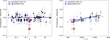 |
Fig. 9 Photospheric versus CI chondrite abundance differences as a function of atomic number, Z (left), and 50% condensation temperature, Tc (right), with photospheric abundances from Asplund et al. (2021) and Amarsi et al. (2025, ‘AAG21/A25’). Silver is circled in red, and the recommended solar silver abundance was used to update AAG21. Weighted linear regressions are overplotted. |
4.4 Comparison with previous results for the Sun and CI chondrites
In Figs. 5 and 6 of Asplund et al. (2021), the authors show a comparison of the recommended solar photospheric abundances with those from CI chondrites. Out of these elements, silver is a nominal >2σ outlier. The authors adopted the 3D LTE solar photospheric silver abundance from Grevesse et al. (2015) of log εAg = 0.96 ± 0.10. Our goal is to update the solar photospheric abundance they used with the presently determined 3D-non-LTE silver abundance and see how it affects these abundance trends.
We update the plots of Asplund et al. (2021) by showing the new recommended 3D-non-LTE silver abundance in Fig. 9. Our plots show elements for which the combined (photospheric and meteoritic) abundance uncertainties are less than 0.15 dex. We include the updated 3D-non-LTE sulphur abundance from Amarsi et al. (2025, which is referred to as ‘AAG21/A25’ in the legends). In the left panel of Fig. 9, we can see that the new silver abundance reduces the difference between the photospheric and meteoritic abundance from –0.25 to –0.06 dex. This reflects the 0.19 dex difference between our recommended solar silver abundance and that of Grevesse et al. (2015) ; see our Sect. 4.3. The photospheric value is now consistent with the meteoritic value to within the estimated uncertainties.
The right panel of Fig. 9 shows the difference between the photospheric and meteoritic values as a function of 50% of the equilibrium condensation temperature at a pressure of 10 4 bar for a solar-composition gas. For the CI chondrites, the values are from Lodders (2021), and we converted them to the solar scale using silicon as the reference element. The 50% equilibrium condensation temperatures were taken from Wood et al. (2019), in which there are updates of the order several hundred kelvin for the moderately volatile elements (such as silver) compared to the often used dataset of Lodders (2003). In the plot, elements whose solar abundances are derived based on a full 3D non-LTE analysis are highlighted by darker colours. These elements are Na, Mg, Al, Si, K, Ca, Fe, and Ba (see Table 1 of Asplund et al. 2021). A linear fit was applied to this 3D-non-LTE subset, taking into account the uncertainties (error bars). Changing the reference element would shift all the points up or down, but it would not affect the fitted gradient.
Whether the differences between the composition of the solar photosphere and of the CI chondrites are a real effect (as suggested by, e.g. Gonzalez et al. 2010; Desch et al. 2018, and Jurewicz et al. 2024) or a result of inaccuracies in the solar spectroscopy (e.g. Lodders et al. 2025) is still debated. What we see from the Asplund et al. (2021) results (referred to as ‘AAG21/A25-L21’ in the figure) is that there is a slight trend in the abundance difference as a function of the condensation temperature. Specifically, with silicon as the reference element, the moderately volatile elements (500 ≲ Tc ≲ 1250 K) are slightly depleted in the Sun, while the refractory elements (Tc ≳ 1370 K) are enhanced in the Sun; the elements in the middle (including silicon with Tc = 1314 K) agree well between the Sun and meteorites. Silver is a moderately volatile element, with Tc = 699 K. When we updated the photospheric silver abundance with our recommended abundance and included the estimated uncertainty on the weighted mean abundance, silver fell into line with the other elements that are based on a full 3D-non-LTE analysis. Refining the analysis so as to reduce the uncertainty below 0.08 dex (see discussion in Sect. 4.3) would be worthwhile to help verify the presence or absence of any systematic differences between the solar and meteoritic abundances.
5 Conclusions
We present a model atom for Ag I and performed a full 3D non-LTE analysis of the solar Ag I resonance lines for the first time. The model atom was built from physically motivated, carefully curated radiative and collisional data. For bound-bound transitions, we supplemented the limited set of experimental oscillator strengths with new calculations. Inelastic hydrogen collisions were computed using a combined asymptotic and free-electron approach to provide a complete dataset.
Because no non-LTE reference calculations for silver exist in the literature, we assessed the robustness of our model through targeted sensitivity tests. The largest sensitivities arise from the hydrogen collisional excitation rates and from the treatment of background opacity in lines overlapping the Ag I diagnostic resonance features, with the hydrogen collision data remaining the dominant caveat. As an additional check, we compared abundances inferred from disc-centre intensity and disc-integrated flux equivalent widths; their close agreement suggests that the adopted hydrogen collision rates do not introduce significant errors.
We find that departures from LTE are driven by the two diagnostic Ag I resonance lines at 328 and 338 nm, leading to overexcitation and overionisation from the ground level and weakening the lines in non-LTE relative to LTE. The 3D effect reinforces this, further reducing the line strengths. The coupling of the 3D and non-LTE effects produces large positive abundance corrections, Δ1(3N – 1L) = +0.28 and ΔF(3N – 1L) = +0.29 dex. Since the non-LTE effect dominates over the 3D effect, a 1D non-LTE treatment provides a much closer approximation to the full 3D non-LTE result than both 1D LTE and 3D LTE.
Using revised equivalent-width measurements of the 328 and 338 nm lines, we re-evaluated the solar silver abundance relative to the 3D LTE value from Grevesse et al. (2015). We recommend log εAg = 1.15 ± 0.08 in 3D non-LTE, with measurement and modelling uncertainties added in quadrature. This is 0.19 dex higher than the previous 3D LTE value (0.96 ± 0.10 dex). The difference is driven by a positive 3D non-LTE versus 3D LTE abundance correction, which is offset by downwards revisions to the equivalent widths of the two Ag I lines.
The revised solar abundance resolves 0.19 dex of the 0.25 dex discrepancy between the solar photospheric and CI chondrite silver abundances reported by Asplund et al. (2021), where the photospheric value appeared significantly underestimated. The residual 0.06 dex discrepancy is consistent with what has been found for other moderately volatile elements and may reflect an intrinsic bias in CI chondrites (e.g. Jurewicz et al. 2024; Amarsi et al. 2025). To confirm this, it would be worthwhile to refine the analysis presented here so as to obtain a more precise measurement of the solar silver abundance.
We also provide non-LTE departure coefficients2 for dwarfs and giants across the MARCS grid of 1D model atmospheres (Gustafsson et al. 2008). Given that the 3D and non-LTE effects act in the same direction (at least for the Sun), a 1D non-LTE approach is expected to be more realistic than 1D LTE for late-type stars. These departure coefficients can therefore be combined with 1D LTE spectrum-synthesis codes such as SME (Piskunov & Valenti 2017) and PySME (Wehrhahn et al. 2023) to improve the accuracy of stellar silver abundance analyses.
Finally, we predicted that the 3D non-LTE versus 1D LTE abundance corrections for the Ag I 328 and 338 nm resonance lines would become increasingly positive towards lower [Fe/H]. As for neutral iron (e.g. Amarsi et al. 2016), the overexcitation and overionisation mechanism should be strengthened as metalline opacity decreases, enhancing the UV radiation field. This may be amplified further by the typically steeper temperature gradients in metal-poor 3D models. A likely consequence is that the inferred [Ag/Fe] versus [Fe/H] may be steeper in 3D non-LTE than in 1D LTE analyses of dwarfs - for example those of Hansen & Primas (2011) - particularly if the AgI corrections exceed those affecting Fe I. We will quantify and discuss these effects in a subsequent paper.
Data availability
The Ag + H rate coefficients are available at https://doi.org/10.5281/zenodo.20038646. The 1D non-LTE departure coefficients across the MARCS model atmosphere grid are available at https://doi.org/10.5281/zenodo.20037437.
Acknowledgements
We thank the referee for suggestions that helped improve the analysis and manuscript. We thank Dan Kiselman for providing helpful advice about solar observations. A.M.A. acknowledges support from the Swedish Research Council (VR 2020-03940, VR 2025-05167) and from the Crafoord Foundation via the Royal Swedish Academy of Sciences (CR 2024-0015). The computations were enabled by resources at the National Supercomputing Centre (NSC, Tetralith cluster) provided by the National Academic Infrastructure for Supercomputing in Sweden (NAISS), partially funded by the Swedish Research Council through grant agreement no. 2022-06725. P.J. acknowledges support from the Swedish Research Council (VR 2023-05367). B.K.S. acknowledges ANRF grant no. CRG/2023/002558 and Department of Space, Government of India for financial supports.
References
- Allen, C. W. 1973, Astrophysical Quantities, 3rd edn. (London: University of London, Athlone Press) [Google Scholar]
- Allende Prieto, C., Asplund, M., & Fabiani Bendicho, P. 2004, A&A, 423, 1109 [NASA ADS] [CrossRef] [EDP Sciences] [Google Scholar]
- Amarsi, A. M. 2015, MNRAS, 452, 1612 [NASA ADS] [CrossRef] [Google Scholar]
- Amarsi, A. M., Lind, K., Asplund, M., Barklem, P. S., & Collet, R. 2016, MNRAS, 463, 1518 [NASA ADS] [CrossRef] [Google Scholar]
- Amarsi, A. M., Barklem, P. S., Asplund, M., Collet, R., & Zatsarinny, O. 2018a, A&A, 616, A89 [NASA ADS] [CrossRef] [EDP Sciences] [Google Scholar]
- Amarsi, A. M., Nordlander, T., Barklem, P. S., et al. 2018b, A&A, 615, A139 [NASA ADS] [CrossRef] [EDP Sciences] [Google Scholar]
- Amarsi, A. M., Ogneva, D., Buldgen, G., et al. 2024, A&A, 690, A128 [NASA ADS] [CrossRef] [EDP Sciences] [Google Scholar]
- Amarsi, A. M., Li, W., Grevesse, N., & Jurewicz, A. J. G. 2025, A&A, 703, A35 [NASA ADS] [CrossRef] [EDP Sciences] [Google Scholar]
- Asplund, M., Nordlund, Â., Trampedach, R., Allende Prieto, C., & Stein, R. F. 2000, A&A, 359, 729 [NASA ADS] [Google Scholar]
- Asplund, M., Grevesse, N., Sauval, A. J., & Scott, P. 2009, ARA&A, 47, 481 [CrossRef] [Google Scholar]
- Asplund, M., Amarsi, A. M., & Grevesse, N. 2021, A&A, 653, A141 [NASA ADS] [CrossRef] [EDP Sciences] [Google Scholar]
- Barklem, P. S. 2016a, A&A Rev., 24, 9 [Google Scholar]
- Barklem, P. S. 2016b, Phys. Rev. A, 93, 042705 [NASA ADS] [CrossRef] [Google Scholar]
- Barklem, P. S. 2017a, Phys. Rev. A, 95, 069906 [Google Scholar]
- Barklem, P. S. 2017b, Astrophysics Source Code Library [record ascl:1701.005] [Google Scholar]
- Barklem, P. S., Piskunov, N., & O’Mara, B. J. 2000, A&AS, 142, 467 [NASA ADS] [Google Scholar]
- Botnen, A., & Carlsson, M. 1999, Astrophys. Space Sci. Lib., 240, 379 [NASA ADS] [CrossRef] [Google Scholar]
- Caffau, E., Ludwig, H.-G., Steffen, M., Freytag, B., & Bonifacio, P. 2011, Sol. Phys., 268, 255 [Google Scholar]
- Caliskan, S., Grumer, J., & Amarsi, A. M. 2024, J. Phys. B Atom. Mol. Phys., 57, 055003 [Google Scholar]
- Caliskan, S., Amarsi, A. M., Racca, M., et al. 2025, A&A, 696, A210 [NASA ADS] [CrossRef] [EDP Sciences] [Google Scholar]
- Carlsson, J., Jönsson, P., & Sturesson, L. 1990, Z. Phys. D, 16, 87 [Google Scholar]
- Civiš, S., Matulková, I., Cihelka, J., et al. 2010, Phys. Rev. A, 82, 022502 [Google Scholar]
- Collet, R., Nordlund, Â., Asplund, M., Hayek, W., & Trampedach, R. 2018, MNRAS, 475, 3369 [NASA ADS] [CrossRef] [Google Scholar]
- Delbouille, L., Roland, G., & Neven, L. 1973, Atlas photometrique du spectre solaire de [lambda] 3000 a [lambda] 10000 (Liège: Universite de Liège) [Google Scholar]
- Desch, S. J., Kalyaan, A. O’D., & Alexander, C. M. 2018, ApJS, 238, 11 [NASA ADS] [CrossRef] [Google Scholar]
- Dravins, D. 1982, ARA&A, 20, 61 [Google Scholar]
- Farouqi, K., Kratz, K.-L., Mashonkina, L. I., et al. 2009, ApJ, 694, L49 [NASA ADS] [CrossRef] [Google Scholar]
- Feller, A., Gandorfer, A., Grauf, B., et al. 2025, Sol. Phys., 300, 65 [Google Scholar]
- François, P., Depagne, E., Hill, V., et al. 2007, A&A, 476, 935 [Google Scholar]
- Froese Fischer, C., Gaigalas, G., Jönsson, P., & Bieron, J. 2019, Comp. Phys. Commun., 237, 184 [Google Scholar]
- Gonzalez, G., Carlson, M. K., & Tobin, R. W. 2010, MNRAS, 407, 314 [NASA ADS] [CrossRef] [Google Scholar]
- Goriely, S. 1999, A&A, 342, 881 [NASA ADS] [Google Scholar]
- Gray, D. F. 2022, The Observation and Analysis of Stellar Photospheres (Cambridge: Cambridge University Press) [Google Scholar]
- Grevesse, N., Scott, P., Asplund, M., & Jacques Sauval, A. 2015, A&A, 573, A27 [NASA ADS] [CrossRef] [EDP Sciences] [Google Scholar]
- Gustafsson, B., Edvardsson, B., Eriksson, K., et al. 2008, A&A, 486, 951 [NASA ADS] [CrossRef] [EDP Sciences] [Google Scholar]
- Hansen, C. J., & Primas, F. 2011, A&A, 525, L5 [NASA ADS] [CrossRef] [EDP Sciences] [Google Scholar]
- Hansen, C. J., Primas, F., Hartman, H., et al. 2012, A&A, 545, A31 [NASA ADS] [CrossRef] [EDP Sciences] [Google Scholar]
- Hayek, W., Asplund, M., Collet, R., & Nordlund, Â. 2011, A&A, 529, A158 [NASA ADS] [CrossRef] [EDP Sciences] [Google Scholar]
- Honda, S., Aoki, W., Ishimaru, Y., Wanajo, S., & Ryan, S. G. 2006, ApJ, 643, 1180 [NASA ADS] [CrossRef] [Google Scholar]
- Huang, P., Zhou, Z., Cui, W., et al. 2025, ApJ, 991, 112 [Google Scholar]
- Jönsson, P., Sahoo, B. K., Caliskan, S., & Amarsi, A. M. 2026, A&A, 709, A31 [NASA ADS] [CrossRef] [EDP Sciences] [Google Scholar]
- Jurewicz, A. J. G., Amarsi, A. M., Burnett, D. S., & Grevesse, N. 2024, Meteor. Planet. Sci., 59, 3193 [Google Scholar]
- Kaulakys, B. 1991, J. Phys. B Atom. Mol. Phys., 24, L127 [Google Scholar]
- Korpi-Lagg, A., Gandorfer, A., Solanki, S. K., et al. 2025, Sol. Phys., 300, 75 [Google Scholar]
- Kramida, A., Yu. Ralchenko, Reader, J., & and NIST ASD Team. 2022, NIST Atomic Spectra Database (ver. 5.10). [Online]. National Institute of Standards and Technology, Gaithersburg, MD [Google Scholar]
- Kratz, K.-L., Farouqi, K., Pfeiffer, B., et al. 2007, ApJ, 662, 39 [NASA ADS] [CrossRef] [Google Scholar]
- Kurucz, R. L. 2017, Canadian J. Phys., 95, 825 [NASA ADS] [CrossRef] [Google Scholar]
- Lagae, C., Amarsi, A. M., Rodríguez Díaz, L. F., et al. 2023, A&A, 672, A90 [NASA ADS] [CrossRef] [EDP Sciences] [Google Scholar]
- Leenaarts, J., & Carlsson, M. 2009, ASP Conf. Ser., 415, 87 [Google Scholar]
- Lind, K., & Amarsi, A. M. 2024, ARA&A, 62, 475 [Google Scholar]
- Lind, K., Amarsi, A. M., Asplund, M., et al. 2017, MNRAS, 468, 4311 [NASA ADS] [CrossRef] [Google Scholar]
- Liu, Y. P., Gao, C., Zeng, J. L., Yuan, J. M., & Shi, J. R. 2014, ApJS, 211, 30 [Google Scholar]
- Lodders, K. 2003, ApJ, 591, 1220 [Google Scholar]
- Lodders, K. 2021, Space Sci. Rev., 217, 44 [NASA ADS] [CrossRef] [Google Scholar]
- Lodders, K., Bergemann, M., & Palme, H. 2025, Space Sci. Rev., 221, 23 [Google Scholar]
- Magic, Z., Collet, R., Asplund, M., et al. 2013, A&A, 557, A26 [NASA ADS] [CrossRef] [EDP Sciences] [Google Scholar]
- Massey, H. S. W. 1949, Rep. Prog. Phys., 12, 248 [Google Scholar]
- Montes, F., Beers, T. C., Cowan, J., et al. 2007, ApJ, 671, 1685 [NASA ADS] [CrossRef] [Google Scholar]
- Moore, C. E., Minnaert, M. G. J., & Houtgast, J. 1966, The Solar Spectrum 2935 A to 8770 A (USA: National Bureau of Standards Monograph) [Google Scholar]
- Nordlund, A., Spruit, H. C., Ludwig, H.-G., & Trampedach, R. 1997, A&A, 328, 229 [Google Scholar]
- Ott, U., & Kratz, K.-L. 2008, New Astron. Rev., 52, 396 [Google Scholar]
- Piskunov, N., & Valenti, J. A. 2017, A&A, 597, A16 [NASA ADS] [CrossRef] [EDP Sciences] [Google Scholar]
- Piskunov, N. E., Kupka, F., Ryabchikova, T. A., Weiss, W. W., & Jeffery, C. S. 1995, A&AS, 112, 525 [Google Scholar]
- Prantzos, N., Abia, C., Cristallo, S., Limongi, M., & Chieffi, A. 2020, MNRAS, 491, 1832 [Google Scholar]
- Prsa, A., Harmanec, P., Torres, G., et al. 2016, AJ, 152, 41 [NASA ADS] [CrossRef] [Google Scholar]
- Roederer, I. U., Cowan, J. J., Karakas, A. I., et al. 2010, ApJ, 724, 975 [NASA ADS] [CrossRef] [Google Scholar]
- Ross, J. E., & Aller, L. H. 1972, Sol. Phys., 25, 30 [Google Scholar]
- Rutten, R. J. 2003, Radiative Transfer in Stellar Atmospheres, 8th edn. (The Netherlands: Utrecht University) [Google Scholar]
- Sahoo, B. K., Jönsson, P., & Gaigalas, G. 2025, Phys. Rev. A, 112, 012809 [Google Scholar]
- Seaton, M. J. 1962, Proc. Phys. Soc., 79, 1105 [NASA ADS] [CrossRef] [Google Scholar]
- Si, R., Li, Y., Wang, K., et al. 2025, Comp. Phys. Commun., 312, 109604 [Google Scholar]
- Sneden, C., Cowan, J. J., & Gallino, R. 2008, Ann. Rev. Astron. Astrophys., 46, 241 [Google Scholar]
- Stein, R. F., Nordlund, Â., Collet, R., & Trampedach, R. 2024, ApJ, 970, 24 [NASA ADS] [CrossRef] [Google Scholar]
- van Regemorter, H. 1962, ApJ, 136, 906 [NASA ADS] [CrossRef] [Google Scholar]
- Wanajo, S., & Ishimaru, Y. 2006, Nucl. Phys. A, 777, 676 [Google Scholar]
- Wehrhahn, A., Piskunov, N., & Ryabchikova, T. 2023, A&A, 671, A171 [NASA ADS] [CrossRef] [EDP Sciences] [Google Scholar]
- Wood, B. J., Smythe, D. J., & Harrison, T. 2019, Am. Mineral., 104, 844 [NASA ADS] [CrossRef] [Google Scholar]
- Wu, X., Wang, L., Shi, J., Zhao, G., & Grupp, F. 2015, A&A, 579, A8 [NASA ADS] [CrossRef] [EDP Sciences] [Google Scholar]
- Zhou, Y., Amarsi, A. M., Aguirre Bϕrsen-Koch, V., et al. 2023, A&A, 677, A98 [NASA ADS] [CrossRef] [EDP Sciences] [Google Scholar]
log εAg ≡ log10 NAg/NH + 12.
All Tables
All Figures
|
Fig. 1 Grotrian diagrams for Ag I illustrating the model atom. The transitions highlighted in blue correspond to the two Ag I diagnostic lines analysed in this work (vacuum wavelengths). The horizontal dotted line marks the silver ionisation limit. |
| In the text | |
|
Fig. 2 Top and middle : non-LTE contribution functions (CFs) to the line depression in the vertical intensity (e.g. Amarsi 2015) for the two diagnostic Ag I lines as a function of vertical optical depth. The contours show the distributions in the 3D model’s solar atmosphere, and the CF in 1D and (3D) are overplotted. All are normalised to the maximum of the 1D LTE CF of the 328 nm line. Bottom : temperature stratification of the 1D, (3D), and 3D model solar atmospheres. |
| In the text | |
|
Fig. 3 Departure coefficients for seven energy levels of Ag I (in increasing excitation energy from left to right) and the ground level of Ag II. The contours show the distributions in the 3D model’s solar atmosphere. The departure coefficients calculated in the (3D) and 1D models are overplotted. |
| In the text | |
|
Fig. 4 Synthetic line profiles of the diagnostic Ag I lines computed in LTE and non-LTE using different solar model atmospheres. No macroturbulence was added to the lines. |
| In the text | |
|
Fig. 5 Photoionisation cross-sections for neutral copper from the ground (3d104s; left) and second excited (3d104p; right) states. The black curves show the R-matrix cross-sections from Liu et al. (2014), while the blue curve shows the hydrogenic approximation; the dashed blue curves indicate the hydrogenic cross-sections shifted by ±1 dex. |
| In the text | |
|
Fig. 6 Comparison of newly calculated MCDHF+RCI oscillator strengths, with oscillator strengths from Civiš et al. (2010) based on the FMP approach. |
| In the text | |
|
Fig. 7 Changes in (3D) non-LTE equivalent widths of the two Ag I diagnostic lines when varying atomic data in the model atom and the background lines (‘test’) compared to the fiduciary model. |
| In the text | |
|
Fig. 8 Fits to Liège disc-centre intensity spectrum, with 3D LTE spectrum synthesis and the VALD line list. The shaded black area reflects the uncertainty in placing the continuum. The shaded blue area shows the equivalent width of the pure Ag I line. Left and middle : synthesis of Ag I 328 nm line, omitting and including a predicted Fe I blend, respectively; the recommended equivalent width for this line in Table 1 is based on the mean of these two results. |
| In the text | |
|
Fig. 9 Photospheric versus CI chondrite abundance differences as a function of atomic number, Z (left), and 50% condensation temperature, Tc (right), with photospheric abundances from Asplund et al. (2021) and Amarsi et al. (2025, ‘AAG21/A25’). Silver is circled in red, and the recommended solar silver abundance was used to update AAG21. Weighted linear regressions are overplotted. |
| In the text | |
Current usage metrics show cumulative count of Article Views (full-text article views including HTML views, PDF and ePub downloads, according to the available data) and Abstracts Views on Vision4Press platform.
Data correspond to usage on the plateform after 2015. The current usage metrics is available 48-96 hours after online publication and is updated daily on week days.
Initial download of the metrics may take a while.