| Issue |
A&A
Volume 687, July 2024
|
|
|---|---|---|
| Article Number | A5 | |
| Number of page(s) | 14 | |
| Section | Astrophysical processes | |
| DOI | https://doi.org/10.1051/0004-6361/202347698 | |
| Published online | 24 June 2024 | |
Titanium abundances in late-type stars
II. Grid of departure coefficients and application to a sample of 70 000 stars
1
Department of Astronomy, Stockholm University, AlbaNova University Centre, Roslagstullsbacken, 106 91 Stockholm, Sweden
e-mail: This email address is being protected from spambots. You need JavaScript enabled to view it.
2
Theoretical Astrophysics, Department of Physics and Astronomy, Uppsala University, Box 516 751 20 Uppsala, Sweden
Received:
10
August
2023
Accepted:
20
February
2024
Abstract
Context. Rapidly growing datasets from stellar spectroscopic surveys are providing unprecedented opportunities to analyse the chemical evolution history of our Galaxy. However, spectral analysis requires accurate modelling of synthetic stellar spectra for late-type stars, for which the assumption of local thermodynamic equilibrium (LTE) has been shown to be insufficient in many cases. Errors associated with LTE can be particularly large for Ti I, which is susceptible to over-ionisation, particularly in metal-poor stars.
Aims. The aims of this work are to study and quantify the 1D non-LTE effects on titanium abundances across the Hertzsprung-Russell diagram for a large sample of stars.
Methods. A large grid of departure coefficients, βν, were computed on standard MARCS model atmospheres. The grid extends from 3000 K to 8000 K in Teff, −0.5 dex to +5.5 dex in log g, and −5.0 to +1.0 in [Fe/H], with non-LTE effects in this grid reaching up to 0.4 dex. This was used to compute abundance corrections that were subsequently applied to the LTE abundances of over 70 000 stars selected from the GALAH survey in addition to a smaller sample of literature Keck data for metal-poor dwarfs.
Results. The non-LTE effects grow towards lower [Fe/H], lower log g, and higher Teff, with a minimum and maximum ΔA(Ti)Ti I of 0.02 and 0.19 in the GALAH sample. For metal-poor giants, the non-LTE modelling reduces the average ionisation imbalance (ΔI−II) from −0.11 dex to −0.01 dex at [Fe/H] = −1.7, and the enhancement in titanium abundances from Ti I lines results in a [Ti/Fe] versus [Fe/H] trend that more closely resembles the behaviour of Ti II at low metallicities. At higher metallicities, the results are limited by the precision of the GALAH DR3 LTE abundances and the effects are within the errors. For the most metal-poor dwarfs from the Keck sample, the average ionisation imbalance increases from −0.1 dex to +0.2 dex, a shortcoming that is consistent with previous 1D non-LTE studies and which we speculate could be related to 3D effects.
Conclusions. Non-LTE effects on titanium abundances are significant. Neglecting them may alter our understanding of Galactic chemical evolution. We have made our grid of departure coefficients publicly available, with the caveat that the Ti abundances of metal-poor dwarfs need further study in 3D non-LTE.
Key words: atomic processes / line: formation / radiative transfer / stars: abundances / Galaxy: abundances
© The Authors 2024
 Open Access article, published by EDP Sciences, under the terms of the Creative Commons Attribution License (https://creativecommons.org/licenses/by/4.0), which permits unrestricted use, distribution, and reproduction in any medium, provided the original work is properly cited.
This article is published in open access under the Subscribe to Open model. This email address is being protected from spambots. You need JavaScript enabled to view it. to support open access publication.
1. Introduction
Data from increasingly expansive stellar spectroscopic surveys have facilitated the advancement of our understanding of galactic chemical evolution (GCE) on a large scale (Jofré et al. 2019). The imminent influx of new data from surveys such as WEAVE (Dalton et al. 2018); weave and 4MOST (de Jong et al. 2019), which will gather of the order of ∼107 high-resolution spectra, will set the stage for unprecedented investigations of the stellar content in our Galaxy.
However, the impact and reliability of such studies are contingent on the accuracy of the applied spectral analysis methods and the underlying modelling of the spectral absorption lines. Local thermodynamic equilibrium (LTE) is a common assumption in the modelling of spectral lines in late-type stars, including our Sun. In the regime of LTE, collisional transitions dominate over radiative ones, and as such the populations of excited and ionised states can be described by the Saha and Boltzmann distributions (Mihalas & Athay 1973; Hubeny & Mihalas 2015). This simplification offers the advantage of fast computation times, which is especially important when analysing large datasets with many spectra. However, this convenience comes at the cost of ignoring potentially important physics.
In the case of titanium, previous 1D LTE work has demonstrated that abundances depend heavily on the diagnostic species: neutral or singly ionised. These so-called ionisation imbalances can be particularly severe in metal-poor stars (Gratton & Sneden 1991). For example, 1D LTE analyses of the metal-poor giant HD122563 have an ionisation imbalance of ΔI−II = −0.4 to −0.45 dex (Sitnova et al. 2020; Mallinson et al. 2022).
Non-LTE analyses have been shown to affect and often reduce this ionisation imbalance in many cases (Bergemann 2011; Sitnova et al. 2016, 2020; Mallinson et al. 2022), with the exception of metal-poor dwarfs. Departures from LTE can be taken into account by solving for the statistical equilibrium (e.g. Rutten 2003). This allows external radiation to impact the local medium, which is vital for the accurate modelling of Ti I; it is the minority species in late-type stars, and with an ionisation energy of 6.8 eV, it has a number of continua in the blue, making it sensitive to over-ionisation. These effects are enhanced in metal-poor stars due to the lack of free electrons from metals such that there are fewer electron collisions to bring Ti I to LTE, and because there is less UV opacity and consequently a larger over-ionising flux. These effects on Ti I do not strongly impact the Ti II lines, however, given that that Ti II is typically the majority species in late-type stars; Ti II also has a higher ionisation energy of 13.6 eV, which prohibits it from experiencing analogous over-ionisation effects.
Inelastic hydrogen collisions are typically a source of large uncertainty in non-LTE calculations, especially for metal-poor stars (Barklem 2016a). Past studies, such as Bergemann (2011) and Sitnova et al. (2016), have carried out non-LTE calculations for titanium using the Drawin recipe for hydrogen collisions (Steenbock & Holweger 1984; Lambert 1993), while more recent studies (e.g. Sitnova et al. 2020; Mallinson et al. 2022) have improved upon this by employing the asymptotic models of Belyaev et al. (2017) and Belyaev & Voronov (2018). Mallinson et al. (2022) also implemented a more extensive model atom and more recent data from Grumer & Barklem (2020) based on the asymptotic model of Barklem (2016b), combined with the recipe from Kaulakys (1991) as suggested in Amarsi et al. (2018, 2019).
The calculations in Sitnova et al. (2020) and Mallinson et al. (2022) show improvements in the ionisation balance in metal-poor giants, in the latter case reducing the ionisation imbalance of HD122563 from ΔI−II = −0.45 dex in LTE to ΔI−II = −0.16 dex in non-LTE. However, for the standard dwarf and subgiant stars considered in Mallinson et al. (2022), departures from LTE appeared to make the ionisation imbalance more severe. Nevertheless, that small-scale study of a few standard stars was not sufficient to conclusively assess the impact of non-LTE modelling across a broad range of parameter space, especially given that 1D hydrostatic model atmospheres were employed in combination with non-spectroscopic stellar parameters.
In this work we aim to more thoroughly study and quantify the 1D non-LTE effects on titanium abundances via the analysis of a large dataset. Following Amarsi et al. (2020), we constructed a grid of departure coefficients1 (Sect. 2) and used it to correct line-by-line LTE titanium abundances for 70 347 stars (Sect. 3.1) selected from the GALAH survey (Martell et al. 2017; Buder et al. 2021) and 13 metal-poor stars observed with Keck (Sneden et al. 2023). We used the results to assess the impact of our non-LTE modelling on titanium ionisation imbalances as well as on our understanding of its Galactic evolution (Sect. 3). We present our overall conclusions in Sect. 4.
2. Method
2.1. Model atom
The model atom used in this work is based on that constructed in Mallinson et al. (2022), and the full details are presented therein. The model contains 459 Ti I levels, 127 Ti II levels, and the ground state of Ti III (587 levels in total). All fine structure was collapsed. All Ti I and Ti II lines were radiatively coupled to the target ground states of the next ionisation stage. In this work the model contains 5026 bound-bound radiative transitions, and the wavelength resolution of these lines was reduced such that the atom contained 63 thousand frequency points overall, compared to the 157 thousand in Mallinson et al. (2022); this had no noticeable impact on final abundances. Inelastic collisions with free electrons were based on van Regemorter (1962) and Cox (2000), and inelastic collisions with neutral hydrogen were based on Grumer & Barklem (2020) and Kaulakys (1991) for Ti I, and on Sitnova et al. (2020) for Ti II.
2.2. Grid of departure coefficients with Balder
The departure coefficient, βi, for a level i is the ratio of populations between LTE and non-LTE:
 (1)
(1)
These departure coefficients for titanium were calculated in the same way as discussed in Amarsi et al. (2022) for iron, using the MPI-parallelised non-LTE radiative transfer code Balder, which is a modified version of Multi3D (Leenaarts & Carlsson 2009). The equation of state and background bound-bound, bound-free, and free-free opacities were calculated with the Blue package (Amarsi et al. 2016). Details of the included species are provided in Zhou et al. (2023). In particular, Thomson scattering from electrons, and Rayleigh scattering on the red wing of Ly-α, were included, while the opacity from background lines was treated in pure absorption.
As described in Amarsi et al. (2020, 2022), the calculations were carried out for 3756 MARCS model atmospheres (Gustafsson et al. 2008) spanning 3000 K to 8000 K in Teff, −0.5 dex to 5.5 dex in log g, and −5.0 dex to +1.0 dex in [Fe/H]. Plane-parallel models with microturbulence ξt = 1.0 km s−1 were used for log g ≥ 4.0, and spherical models with solar mass and ξt = 2.0 km s−1 were used otherwise for consistency with Amarsi et al. (2021). For each of these grid nodes, the calculations with Balder were carried out for different choices of titanium abundance, with [Ti/Fe] ∈ [ − 2.0, −1.0, −0.5, 0.0, +0.5, +1.0, +2.0]. The microturbulence used in Balder was fixed to that used for the construction of the model atmosphere, namely ξt = 1.0 km s−1 for log g ≥ 4.0, and ξt = 2.0 km s−1 otherwise.
It should be noted that the model atom adopts level configurations and spectroscopic terms based on those from Kurucz (2016). Following Amarsi et al. (2020), the departure coefficients were mapped from these levels onto those given in NIST (Ralchenko & Kramida 2020).
2.3. Abundance corrections with PySME
The departure coefficients from Sect. 2.2 were constructed in such a way as to be compatible with the spectrum synthesis codes SME and PySME (Wehrhahn et al. 2023). For each Ti line, PySME searches for its upper and lower level in the grid of departure coefficients, and uses them to correct the LTE level populations before synthesising the line with the correct non-LTE line opacity and line source function (Piskunov & Valenti 2017).
As in Lind et al. (2022), PySME was used to generate abundance corrections using the departure coefficients for more values of [Ti/Fe] and ξt. Namely, synthetic spectra were calculated for [Ti/Fe] between −2.0 dex and +2.0 dex in steps of 0.25 dex, and ξt = 1 km s−1 and 2 km s−1. These were performed on a subset of the MARCS model atmospheres; Fig. 1 shows these grid nodes, as well as the selected GALAH stars (described in Sect. 2.4). For a given titanium line, equivalent widths were calculated in LTE and non-LTE and linearly interpolated to generate a grid of abundance corrections shown in Fig. 2. Finally, these abundance corrections were linearly interpolated onto the line-by-line LTE GALAH abundances, as functions of Teff, log g, [Fe/H], ξt, and abundance A(Ti)line, LTE. The star selection is described in Sect. 2.4 and the line selection is described in Sect. 2.5, below.
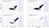 |
Fig. 1. Kiel diagrams showing the values of Teff and log g at which the non-LTE calculations were performed with PySME, as well as the selected GALAH stars for different metallicity ranges. |
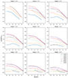 |
Fig. 2. Trend lines showing the non-LTE effects for unsaturated lines (Wred, λ = log(W/λ) < −4.9) of Ti I across a range of stellar parameters. All models shown have ξt = 2 km s−1 and at least two lines from Table 1. |
2.4. GALAH DR3 star selection
This work builds upon the few benchmark stars analysed in Mallinson et al. (2022) and examines a subsample of 70 347 stars, all of which have some measurement of titanium abundance from either Ti I or Ti II (or both), out of the 588 571 stars in GALAH DR3 (Buder et al. 2021). These data contain Teff, log g, and [Fe/H] (both the initial atmospheric and final estimate of abundance, with the latter being used in this work), ξt, and line-by-line LTE titanium abundances, A(Ti)line, LTE. The way in which these parameters were determined are described in Buder et al. (2021). To give a short summary, these parameters were determined by normalising the spectra based on some initial guess, and optimising the stellar parameters. Forming an initial log g by the mass-luminosity relation, Teff, [Fe/H], vbroad, and vrad are optimised with double-sided partial derivatives and χ2, updating log g and vmic with each change, repeating this until the change in χ2 was below 0.001 for each iteration. [Fe/H] was finally redetermined in non-LTE via analysing Fe lines directly (and this value of [Fe/H] is adopted for the present study).
The selected stars are shown in Fig. 1. The selection was made by limiting to those stars with the most reliable parameters and highest signal-to-noise ratio. This was done in several steps. First, only the stars with quality flags of 0 for [Fe/H] and [Ti/Fe] (‘flag_fe_h’, ‘flag_ti_fe’, and ‘flag_ti2_fe’) and the stellar parameter flag ‘flag_sp’ were selected. Secondly, as recommended in the best practices for using the data from the GALAH consortium2, the average signal-to-noise ratio per pixel for the third charged couple device was limited to 30 or above (snr_c3_iraf > 30) for very metal-poor stars ([Fe/H] < −1.5), in order to keep enough low metallicity stars in the sample for a robust analysis, and average signal-to-noise ratio over all lines of S/N > 70 for the stars at higher metallicities. Finally, only stars with at least two lines with a reduced equivalent width Wred, λ = log(Wλ/λ) in LTE between −6.0 < Wred, λ < −4.9 were kept.
2.5. Line selection
As the GALAH reanalysis of absolute abundances, A(Ti), was done on a line-by-line basis, the line-by-line scatter can be used as another diagnostic of the non-LTE modelling. The line selection strongly influences the final results, and care was taken to try to select the best available lines out of those considered by GALAH.
Ti I lines were initially limited to those that are reported as unblended in Heiter et al. (2020) in the Sun and Arcturus, although the 6599.11 Å line was also removed due to a lack of titanium abundance data in the available stars.
In the case of Ti II, no lines were reported as unblended, so lines were instead restricted to those that were reported as uncertain. Of the remaining available lines, 4865.6 Å can be strongly affected by Hβ, causing blending and continuum normalisation, primarily in dwarfs. However, to keep the line list identical for all stars, it was removed entirely. To increase the line list to more than two lines, the least visibly blended line in the Sun and Arcturus that was not examined in Heiter et al. (2020), at 4719.51 Å, was added.
The relative abundances [Ti/H] and [Ti/Fe] were determined on a line-by-line basis using the GALAH abundances, with non-LTE solar corrections applied to their values when in non-LTE. Average values of [Ti/H] were calculated for different species, [Ti/H]Ti I and [Ti/H]Ti II, via a mean of the available lines for a given star weighted by their error. Weak lines and strong lines were cut using the reduced equivalent width criterion of −6.0 < Wred, λ < −4.9. The upper limit prevents the use of saturated lines, which would have both given an under-abundance and increase the sensitivity to microturbulence error. The lower limit reduces the impact of noise fluctuation. The un-normalised weights were given by  , using the uncertainties provided by GALAH. Finally, where illustrated in Sect. 3.1 below, the absolute abundances use the non-LTE line-averaged solar correction: 0.052 dex for Ti I and −0.002 dex for Ti II.
3. Results and discussion
3.1. Non-LTE effects across the Hertzsprung-Russell diagram
Figures 3–6 show the line-averaged non-LTE corrections of Ti I and Ti II as a function of stellar parameters. The non-LTE effects on both species grow in severity towards lower metallicities, lower surface gravities, and higher effective temperatures, qualitatively similar to that found for iron in Lind et al. (2012).
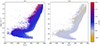 |
Fig. 3. Non-LTE abundance correction for A(Ti)Ti I and A(Ti)Ti II, averaged over lines, for the GALAH sample across the Kiel diagram. |
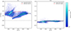 |
Fig. 4. Non-LTE abundance correction for A(Ti)Ti I and A(Ti)Ti II, averaged over lines, as a function of Teff for the GALAH sample. The trends for dwarfs and giants are shown as solid and dashed lines, respectively, using bins of ΔTeff = ±75 K and limited to bins containing at least 30 stars. The colour gradient represents the number of stars per pixel. |
For Ti I, the abundance corrections rise to +0.18 dex on average for giants at [Fe/H] = −2.0 (Fig. 6). The analysis of benchmark stars in Mallinson et al. (2022) suggests that the dwarfs should show a similar trend with [Fe/H] as the giants, namely increasing non-LTE abundance corrections with decreasing metallicity. However, the dwarfs in this sample only extend down to [Fe/H] = −1.0, reflecting the low number of very metal-poor dwarfs in the dataset of Buder et al. (2021). At [Fe/H] = −1.0, the abundance corrections reach +0.08 dex, compared to +0.13 dex for giants at this same metallicity.
The abundance corrections for Ti II are generally much less severe than for Ti I. This is because of the majority status of Ti II: due to the larger number of ions, the effect of over-ionisation by UV radiation is smaller overall, which implies that the assumption of LTE for both dwarfs and giants is a more reasonable one for this species. The corrections are typically −0.02 dex for giants but rising at low metallicities, and consistent with zero for the dwarfs in the GALAH sample. However, at the lowest metallicities around [Fe/H] = −2.0 the abundance corrections reverse sign and tend to become slightly positive (Fig. 6), consistent with Mallinson et al. (2022). It reflects how over-excitation due to radiative pumping becomes increasingly important for this species towards lower metallicities (Sitnova et al. 2020).
Additionally, the impact of titanium abundance itself on the non-LTE corrections for Ti I was investigated in Fig. 7 for benchmark stars from Mallinson et al. (2022). Between −1.00 < [Ti/Fe] < 0.75 the correction changes by only 0.05 dex for the Sun, and 0.09 dex for HD122563. Due to the large difference in abundance, this is not a significant change and within the error of this paper.
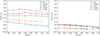 |
Fig. 7. Trend lines showing the non-LTE effects for unsaturated lines (Wred, λ = log(W/λ) < −4.9) of Ti I across five benchmark stars: the Sun (5773, 4.44, 0.00, 1.0), Arcturus (4286, 1.64, −0.53, 1.3), HD84937 (6356, 4.06, −2.06, 1.2), HD140283 (5792, 3.65, −2.36, 1.3), and HD122563 (4636, 1.40, −2.50, 1.8) with parameters of Teff, log g, [Fe/H], and ξt, respectively. |
3.2. Ionisation imbalances
3.2.1. GALAH stars
The difference in the predictions based on Ti I and Ti II is a long-standing problem in studies of titanium abundances, with Ti I predicting lower abundances than Ti II. Neglected non-LTE effects are a contributing factor to this problem (Bergemann 2011). For both dwarfs and giants, the abundance corrections become larger towards lower metallicities for Ti I, while remaining rather close to zero for Ti II.
Consequently, the ionisation imbalance is reduced in non-LTE in giants from the GALAH sample at low metallicities, as shown in Fig. 8. For giants in LTE, the ionisation imbalance reaches on average ΔI−II = −0.11, dex at [Fe/H] ≈ −1.7. In non-LTE, this is reduced to ΔI−II = −0.01, demonstrating a non-LTE impact on the imbalance of 0.10 dex.
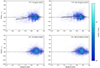 |
Fig. 8. Ionisation imbalance, ΔI−II, of titanium at various metallicities in LTE (left) and non-LTE (right) for giants (upper) and dwarfs (lower) from the GALAH sample. The colour gradient and trend lines are the same as in Fig. 6. |
For dwarfs in the GALAH sample, departures from LTE do not significantly alter the ionisation imbalance on average, with an imbalance of ΔI−II = −0.000 for LTE and ΔI−II = −0.001 in non-LTE, at [Fe/H] ≈ −0.9. It should be noted that this results in a solar abundance correction of 0.05 dex for Ti I and −0.002 dex for Ti II (see Table 1 and Sect. 2.5); the square bracket notation thus hides an ionisation imbalance of around 0.05 dex.
GALAH lines.
3.2.2. Keck stars
Due to the lack of low metallicity dwarfs available in the GALAH data sample, an additional set of stars were taken from Sneden et al. (2023), consisting of 13 dwarfs of the original 37 due to line selection and saturation; the majority of which have a metallicity between −3.0 < [Fe/H] < −2.0, as shown in Fig. 9. The spectra of these stars were obtained with Keck I/HIRES spectrograph (Vogt et al. 1994), and originally used in Boesgaard et al. (2011). The lines available for these stars do not overlap with those in the GALAH data, and the majority instead are below 4000 Å. The inclusion of these lines dramatically reduces the abundance of both species of titanium.
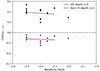 |
Fig. 9. Ionisation imbalance, ΔI−II, of titanium in metal-poor dwarfs and subgiants from the Keck sample (Sneden et al. 2023) in both LTE and non-LTE for the lines shown in Table 2. Trend lines are the same as in Fig. 6. |
In HD84937, Lawler et al. (2013) found a strong reduction in Ti I abundances of around 0.15 − 0.2 dex when moving to the near-UV range of λ = 3100 − 3700 Å. Wood et al. (2013) find similarly for the high excitation energy lines. The overabundance of UV lines in the Ti II line list may result in the heavily positive LTE ionisation imbalance ΔI−II seen in Sneden et al. (2023) that is in disagreement with the expectations from previous work that focused on the longer optical wavelength lines (Bergemann 2011; Sitnova et al. 2020; Mallinson et al. 2022). The cause of this may be related to the Balmer continuum opacity (Wood et al. 2013). In Sneden et al. (2016), the removal of these lines raises the Ti II-based abundance and results in a smaller imbalance, similar to that found for HD84937 in Mallinson et al. (2022).
By including only unsaturated and reasonably strong lines (−6.0 < Wred, λ < −4.8) above this limit (i.e. > 3700 Å, as shown in Table 2), only 13 of the original 34 stars in Sneden et al. (2023) can be analysed. However, this gives the ionisation imbalance for dwarfs at these metallicities a closer agreement with Mallinson et al. (2022) and remains close to 0 in LTE, worsening in non-LTE and prompting 3D analysis to further investigate.
Keck I/HIRES sample of Sneden et al. (2023), with the same layout as Table 1.
3.2.3. 3D impact
The inclusion of 3D effects is a potential solution to the ionisation imbalance of Ti. To estimate its impact in LTE, we employed four snapshots of two 3D STAGGER radiation-hydrodynamic models (Magic et al. 2013). The models pertain to metal-poor dwarfs with Teff = 6000 K, log g = 4.5, [Fe/H] = −3.0 and [Fe/H] = −2.0, respectively. [Ti/Fe] was set to 0.4, and we adopted ξ = 1 km s−1 in the corresponding 1D calculations. The spectral lines listed in Table 2 were computed both in 1D and 3D under LTE conditions using the SCATE (Hayek et al. 2011) code. The mean 3D effects (i.e. 3D minus 1D abundance differences) were found to be −0.41 dex and 0.01 dex for Ti I and Ti II, respectively, in the [Fe/H] = −3 model, and −0.36 dex and −0.05 dex, respectively, in the [Fe/H] = −2 model.
For giants characterised by Teff = 4000 K, log g = 2.0, and [Fe/H] = −2.0, a considerably lesser impact of −0.04 and +0.06 is found for Ti I and Ti II, respectively. These findings align with prior research (Dobrovolskas et al. 2013) that reports a large abundance change in 3D for resonant lines only at around −0.45 dex at [Fe/H] = −3, but that steeply decreases to −0.05 dex in abundance change as the excitation energy increases to 2 eV.
These results underscore the significant influence of 3D effects on Ti I in the inverse direction of non-LTE, offering a potential resolution to the dwarf metallicity discrepancy at lower metallicities. However, the interaction between 3D and non-LTE is not necessarily additive (Lagae et al. 2023) and a full 3D non-LTE investigation would be needed to make strong conclusions.
3.3. Star-by-star scatter
The abundance results in Fig. 10 also suggest a slight reduction in the star-by-star scatter in the [Ti/Fe] versus [Fe/H] plane when departures from LTE are taken into account. This is also illustrated in Fig. 11, where we plot the standard deviation in the [Ti/Fe] versus [Fe/H] plane in different [Fe/H] bins for given titanium lines. There is indeed a slight reduction in the star-by-star scatter, reaching over 0.01 dex for the Ti I4759.27 Å line in low-metallicity giants. As a result, the offset between dwarfs and giants is slightly reduced when comparing the upper left and upper right panels of Fig. 10.
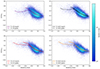 |
Fig. 10. Run of [Ti/Fe] versus [Fe/H] in LTE (left) and non-LTE (right) from Ti I (upper) and Ti II (lower) for the GALAH sample. Trend lines are the same as in Fig. 6. |
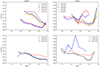 |
Fig. 11. Star-by-star scatter for dwarfs (left) and giants (right) for different lines of Ti I (upper) and Ti II (lower) from the GALAH sample. The colour gradient and the trend lines are the same as in Fig. 6. |
It is plausible that the scatter of these results is dominated by issues with the LTE GALAH abundances. As such, the non-LTE model presented here may lead to a further reduction in the star-by-star and line-by-line scatter when applied to more precise measurements, but no strong conclusion can be made from such small effects.
3.4. Departures from LTE for different stellar parameters
The impact that stellar parameters have on the magnitude of the non-LTE effect is shown in Fig. 2, computed using the MARCS atmospheres at specific grid points with (PySME), and plotted as the average non-LTE impact on A(Ti), averaged over the chosen GALAH Ti I lines. As is found in previous work, a decrease in metallicity increases the magnitude of Δ A(Ti)Ti I in most cases, particularly between −3 < [Fe/H] < 0. Similarly, a decreasing log g results in a larger non-LTE effect as collisional rates – scaling with the number density of both titanium atoms and the ionising impact species – reduce faster than radiative rates, which scales only with the number density of titanium. As seen in Fig. 2, this effect also increases with Teff until around Teff ≈ 6000 K, as the increased number of photons outweigh the increased number and speed of colliders. Beyond this, as with most titanium lines in Sitnova et al. (2016), the increasing temperature begins to reduce the non-LTE effect up to our limit of 7000 K. The exact temperature at which this decline occurs varies with log g and [Fe/H]. Of the available grid points, the most extreme non-LTE effects range from −0.004 (at Teff = 4000 K, log g = 2.5, [Fe/H] = 0.5) to 0.442 dex (at Teff = 5000 K, log g = 1.0, [Fe/H] = − 4.0).
3.5. The Galactic evolution of titanium
Precision measurements of chemical abundances are crucial to accurately interpreting and constraining theories of GCE. While titanium is formally considered an iron peak element, it often behaves as an alpha element in observations (Zhao et al. 2016; Kobayashi et al. 2020). Thus, it is useful in disentangling Galactic components and tracing back their evolution histories. For example, [Ti/Fe] can be used as a chemical tracer to separate the chemical thin and thick discs, stellar halo and accreted stellar populations (e.g. Bensby et al. 2005, 2014; Mashonkina et al. 2019). In addition, the Galactic Anticenter Stellar Structure, or ‘Monoceros Ring’, has been shown to exhibit abundance patterns in [Ti/Fe] and [Y/Fe] that are similar to those of Sagittarius stars and distinct from Milky Way stars, allowing for constraints to be placed on the origin of this structure (Chou et al. 2010).
Interestingly, some recent GCE models show that [Ti/Fe] is under-predicted by ∼0.4 dex over a wide metallicity range when compared to observational data (Kobayashi et al. 2006, 2020; Romano et al. 2010), even in non-LTE (Mashonkina et al. 2019). It has been shown that [Ti/Fe] levels can be increased by including yields from asymmetric 2D models of high-entropy, jet-like ejecta from hypernovae (Maeda & Nomoto 2003; Tominaga 2009) in these GCE models (see model K15, as presented in Sneden et al. 2016; Kobayashi et al. 2020), but high precision measurements of [Ti/Fe] are needed to constrain the parameters of these ejecting supernovae. Notably, the non-LTE corrections presented in this work have shown that average giant [Ti/Fe] abundances measured with Ti I become larger by ∼0.1 dex as compared to 1D-LTE analyses, thereby exacerbating the discrepancy between models and observations, particularly at low metallicities of [Fe/H] < −0.7, but brings Ti I observations to agreement with Ti II as shown in Figs. 10 and 12.
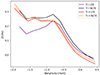 |
Fig. 12. Trend of [Ti/Fe] versus [Fe/H] in LTE and non-LTE from Ti I and Ti II. Based on the binning from Fig. 10 for the GALAH sample, averaged over dwarfs and giants. |
In a study designed to investigate the impact of modelling assumptions on GCE yields, Côté et al. (2017) emphasise the significant influence of the choice of stellar yields on the trends in chemical evolution. With different stellar models within their set of stellar yields, they substantially reduce the titanium underprediction of Côté et al. (2016) and Kobayashi et al. (2020) and successfully replicate an approximately +0.25 enhancement in [Ti/Fe] at low metallicities, within the framework of a one-zone model, and consistent with observations in the Sculptor dwarf galaxy. However, they point out that these abundance trends can be realised through various combinations of input parameters, making it challenging to distinguish among several degenerate models, a caveat that was also described in previous work (Romano & Starkenburg 2013).
Clearly, the abundance trends from these models are highly dependent on the choice of input parameters and the adopted stellar yields. This implies a fundamental limitation in one-zone GCE models, which cannot be overcome by simply increasing the precision of observed abundance data.
Therefore, while the non-LTE corrections reduce the discrepancy between abundances measured using Ti I and Ti II for giants at low metallicities, they are not sufficient to offer further insight needed to constrain GCE models. They nevertheless emphasise the need for improved precision in theoretical yields for these models.
4. Conclusion
This study is the first to investigate the impact of 1D non-LTE effects on titanium abundances across a large sample of stars, building upon previous work that had primarily examined a small number of benchmark stars. It was expected that larger non-LTE effects would be found for Ti I, in metal-poor stars, and in giants: all three of these predictions are confirmed in this investigation. This resulted in a reduced ionisation imbalance for the metal-poor giants, a slight reduction in the disagreement between dwarf and giant titanium abundances at lower metallicities, and a shift in the [Ti/Fe] trend of Ti I to more closely match that of Ti II at low metallicities. This takes observations further away from predictions by some GCE models of titanium (Kobayashi et al. 2020, and references therein). Overall, this suggests that the inclusion of the departure coefficient grid and correcting for non-LTE effects results in more accurate Ti I abundances for giants at lower metallicities, although this is dependent on the line selection.
Due to the small sample of metal-poor dwarfs and the relatively low accuracy of the GALAH sample, the limitations of this analysis are apparent. In Mallinson et al. (2022), metal-poor dwarfs were seen to have their imbalance worsened by the inclusion of non-LTE, a conclusion that is reinforced by our analysis of the Sneden et al. (2023) sample in this work. An investigation of 3D non-LTE effects for Ti in metal-poor stars may shed further light on the problem. Additionally, the low number of lines and their quality – particularly for Ti II – further limit the reliability of these results.
Finally, there were larger departures from LTE towards higher effective temperatures and lower surface gravities, as well as lower metallicities. However, at lower surface gravities of log g < 3.5, increasing the temperature beyond Teff ≈ 5500 K reduced the departures from LTE. Likewise, a lower metallicity can occasionally result in lower non-LTE effects in all lines analysed, primarily at low temperatures and high surface gravity. In summary, we find the non-LTE corrections reach up to +0.41 dex at Teff = 5000 K, log g = 1.0, [Fe/H] = −4.0.
Our grid of departure coefficients is publicly available at https://zenodo.org/record/10753497
Acknowledgments
AMA acknowledges support from the Swedish Research Council (VR 2020-03940). This research was supported by computational resources provided by the Australian Government through the National Computational Infrastructure (NCI) under the National Computational Merit Allocation Scheme and the ANU Merit Allocation Scheme (project y89). This work has made use of the VALD database, operated at Uppsala University, the Institute of Astronomy RAS in Moscow, and the University of Vienna. We thank the PDC Center for High Performance Computing, KTH Royal Institute of Technology, Sweden, for providing access to computational resources and support. JWEM, KL, and KY acknowledge funds from the European Research Council (ERC) under the European Union’s Horizon 2020 research and innovation programme (Grant agreement No. 852977) and funds from Knut and Alice Wallenberg Foundation. We acknowledge Chris Sneden for the sharing of his data and advice in its analysis.
References
- Amarsi, A. M., Lind, K., Asplund, M., Barklem, P. S., & Collet, R. 2016, MNRAS, 463, 1518 [NASA ADS] [CrossRef] [Google Scholar]
- Amarsi, A. M., Barklem, P. S., Asplund, M., Collet, R., & Zatsarinny, O. 2018, A&A, 616, A89 [NASA ADS] [CrossRef] [EDP Sciences] [Google Scholar]
- Amarsi, A. M., Barklem, P. S., Collet, R., Grevesse, N., & Asplund, M. 2019, A&A, 624, A111 [NASA ADS] [CrossRef] [EDP Sciences] [Google Scholar]
- Amarsi, A. M., Lind, K., Osorio, Y., et al. 2020, A&A, 642, A62 [EDP Sciences] [Google Scholar]
- Amarsi, A. M., Grevesse, N., Asplund, M., & Collet, R. 2021, A&A, 656, A113 [NASA ADS] [CrossRef] [EDP Sciences] [Google Scholar]
- Amarsi, A. M., Liljegren, S., & Nissen, P. E. 2022, A&A, 668, A68 [NASA ADS] [CrossRef] [EDP Sciences] [Google Scholar]
- Barklem, P. S. 2016a, A&A Rev., 24, 9 [NASA ADS] [CrossRef] [Google Scholar]
- Barklem, P. S. 2016b, Phys. Rev. A, 93, 042705 [NASA ADS] [CrossRef] [Google Scholar]
- Barklem, P. S., Piskunov, N., & O’Mara, B. J. 2000, A&AS, 142, 467 [NASA ADS] [CrossRef] [EDP Sciences] [Google Scholar]
- Belyaev, A. K., & Voronov, Y. V. 2018, ApJ, 868, 86 [NASA ADS] [CrossRef] [Google Scholar]
- Belyaev, A. K., Yakovleva, S. A., & Kraemer, W. P. 2017, Eur. Phys. J. D, 71, 276 [NASA ADS] [CrossRef] [Google Scholar]
- Bensby, T., Feltzing, S., Lundström, I., & Ilyin, I. 2005, A&A, 433, 185 [NASA ADS] [CrossRef] [EDP Sciences] [Google Scholar]
- Bensby, T., Feltzing, S., & Oey, M. S. 2014, A&A, 562, A71 [NASA ADS] [CrossRef] [EDP Sciences] [Google Scholar]
- Bergemann, M. 2011, MNRAS, 413, 2184 [NASA ADS] [CrossRef] [Google Scholar]
- Boesgaard, A. M., Rich, J. A., Levesque, E. M., & Bowler, B. P. 2011, ApJ, 743, 140 [Google Scholar]
- Buder, S., Sharma, S., Kos, J., et al. 2021, MNRAS, 506, 150 [NASA ADS] [CrossRef] [Google Scholar]
- Chou, M.-Y., Majewski, S. R., Cunha, K., et al. 2010, ApJ, 720, L5 [NASA ADS] [CrossRef] [Google Scholar]
- Côté, B., West, C., Heger, A., et al. 2016, MNRAS, 463, 3755 [CrossRef] [Google Scholar]
- Côté, B., O’Shea, B. W., Ritter, C., Herwig, F., & Venn, K. A. 2017, ApJ, 835, 128 [Google Scholar]
- Cox, A. N. 2000, Allen’s Astrophysical Quantities (New York: AIP Press) [Google Scholar]
- Dalton, G., Trager, S., Abrams, D. C., et al. 2018, SPIE Conf. Ser., 10702, 107021B [Google Scholar]
- de Jong, R. S., Agertz, O., Berbel, A. A., et al. 2019, The Messenger, 175, 3 [NASA ADS] [Google Scholar]
- Dobrovolskas, V., Kučinskas, A., Steffen, M., et al. 2013, A&A, 559, A102 [NASA ADS] [CrossRef] [EDP Sciences] [Google Scholar]
- Gratton, R. G., & Sneden, C. 1991, A&A, 241, 501 [NASA ADS] [Google Scholar]
- Grumer, J., & Barklem, P. S. 2020, A&A, 637, A28 [NASA ADS] [CrossRef] [EDP Sciences] [Google Scholar]
- Gustafsson, B., Edvardsson, B., Eriksson, K., et al. 2008, A&A, 486, 951 [NASA ADS] [CrossRef] [EDP Sciences] [Google Scholar]
- Hayek, W., Asplund, M., Collet, R., & Nordlund, Å. 2011, A&A, 529, A158 [NASA ADS] [CrossRef] [EDP Sciences] [Google Scholar]
- Heiter, U., Lind, K., Bergemann, M., et al. 2020, VizieR Online Data Catalog: J/A+A/645/A106 [Google Scholar]
- Hubeny, I., & Mihalas, D. 2015, Theory of Stellar Atmospheres. An Introduction to Astrophysical Non-equilibrium Quantitative Spectroscopic Analysis (Princeton University Press) [Google Scholar]
- Jin, S., Trager, S. C., Dalton, G. B., et al. 2024, MNRAS, 530, 2688 [NASA ADS] [CrossRef] [Google Scholar]
- Jofré, P., Heiter, U., & Soubiran, C. 2019, ARA&A, 57, 571 [Google Scholar]
- Kaulakys, B. 1991, J. Phys. B: At. Mol. Opt. Phys., 24, L127 [NASA ADS] [CrossRef] [Google Scholar]
- Kobayashi, C., Umeda, H., Nomoto, K., Tominaga, N., & Ohkubo, T. 2006, ApJ, 653, 1145 [NASA ADS] [CrossRef] [Google Scholar]
- Kobayashi, C., Karakas, A. I., & Lugaro, M. 2020, ApJ, 900, 179 [Google Scholar]
- Kurucz, R. L. 2016, Kurucz on-line database of observed and predicted atomic transitions, http://kurucz.harvard.edu/atoms/ [Google Scholar]
- Lagae, C., Amarsi, A. M., Rodríguez Díaz, L. F., et al. 2023, A&A, 672, A90 [NASA ADS] [CrossRef] [EDP Sciences] [Google Scholar]
- Lambert, D. L. 1993, Phys. Scr. T, 47, 186 [CrossRef] [Google Scholar]
- Lawler, J. E., Guzman, A., Wood, M. P., Sneden, C., & Cowan, J. J. 2013, ApJS, 205, 11 [Google Scholar]
- Leenaarts, J., & Carlsson, M. 2009, in The Second Hinode Science Meeting: Beyond Discovery-Toward Understanding, eds. B. Lites, M. Cheung, T. Magara, J. Mariska, & K. Reeves, ASP Conf. Ser., 415, 87 [Google Scholar]
- Lind, K., Bergemann, M., & Asplund, M. 2012, MNRAS, 427, 50 [Google Scholar]
- Lind, K., Nordlander, T., Wehrhahn, A., et al. 2022, A&A, 665, A33 [NASA ADS] [CrossRef] [EDP Sciences] [Google Scholar]
- Maeda, K., & Nomoto, K. 2003, Nucl. Phys. A, 718, 167 [Google Scholar]
- Magic, Z., Collet, R., Asplund, M., et al. 2013, A&A, 557, A26 [NASA ADS] [CrossRef] [EDP Sciences] [Google Scholar]
- Mallinson, J. W. E., Lind, K., Amarsi, A. M., et al. 2022, A&A, 668, A103 [NASA ADS] [CrossRef] [EDP Sciences] [Google Scholar]
- Martell, S. L., Sharma, S., Buder, S., et al. 2017, MNRAS, 465, 3203 [CrossRef] [Google Scholar]
- Mashonkina, L. I., Neretina, M. D., Sitnova, T. M., & Pakhomov, Y. V. 2019, Astron. Rep., 63, 726 [NASA ADS] [CrossRef] [Google Scholar]
- Mihalas, D., & Athay, R. G. 1973, ARA&A, 11, 187 [NASA ADS] [CrossRef] [Google Scholar]
- Piskunov, N., & Valenti, J. A. 2017, A&A, 597, A16 [NASA ADS] [CrossRef] [EDP Sciences] [Google Scholar]
- Ralchenko, Y., & Kramida, A. 2020, Atoms, 8, 56 [NASA ADS] [CrossRef] [Google Scholar]
- Romano, D., & Starkenburg, E. 2013, MNRAS, 434, 471 [Google Scholar]
- Romano, D., Karakas, A. I., Tosi, M., & Matteucci, F. 2010, A&A, 522, A32 [NASA ADS] [CrossRef] [EDP Sciences] [Google Scholar]
- Rutten, R. J. 2003, Radiative Transfer in Stellar Atmospheres (Lecture Notes Utrecht University), 255 [Google Scholar]
- Ryabchikova, T., Piskunov, N., Kurucz, R. L., et al. 2015, Phys. Scr., 90, 054005 [Google Scholar]
- Sitnova, T. M., Mashonkina, L. I., & Ryabchikova, T. A. 2016, MNRAS, 461, 1000 [Google Scholar]
- Sitnova, T. M., Yakovleva, S. A., Belyaev, A. K., & Mashonkina, L. I. 2020, Astron. Lett., 46, 120 [NASA ADS] [CrossRef] [Google Scholar]
- Sneden, C., Cowan, J. J., Kobayashi, C., et al. 2016, ApJ, 817, 53 [NASA ADS] [CrossRef] [Google Scholar]
- Sneden, C., Boesgaard, A. M., Cowan, J. J., et al. 2023, ApJ, 953, 31 [CrossRef] [Google Scholar]
- Steenbock, W., & Holweger, H. 1984, A&A, 130, 319 [NASA ADS] [Google Scholar]
- Tominaga, N. 2009, ApJ, 690, 526 [NASA ADS] [CrossRef] [Google Scholar]
- van Regemorter, H. 1962, ApJ, 136, 906 [NASA ADS] [CrossRef] [Google Scholar]
- Vogt, S. S., Allen, S. L., Bigelow, B. C., et al. 1994, in Instrumentation in Astronomy VIII, eds. D. L. Crawford, & E. R. Craine, SPIE Conf. Ser., 2198, 362 [Google Scholar]
- Wehrhahn, A., Piskunov, N., & Ryabchikova, T. 2023, A&A, 671, A171 [NASA ADS] [CrossRef] [EDP Sciences] [Google Scholar]
- Wood, M. P., Lawler, J. E., Sneden, C., & Cowan, J. J. 2013, ApJS, 208, 27 [NASA ADS] [CrossRef] [Google Scholar]
- Zhao, G., Mashonkina, L., Yan, H. L., et al. 2016, ApJ, 833, 225 [Google Scholar]
- Zhou, Y., Amarsi, A. M., Aguirre Børsen-Koch, V., et al. 2023, A&A, 677, A98 [NASA ADS] [CrossRef] [EDP Sciences] [Google Scholar]
Appendix A: Additional non-LTE effects and microturbulence sensitivity
This appendix contains additional figures where Figure A.1 represents the non-LTE effects for lines as in Fig. 2 but for Ti II, and the impact titanium abundance has on non-LTE effects in benchmark stars. Figures A.2-A.3 shows the impact reduced equivalent width has on microturbulence sensitivity in GALAH stars with their microturbulences replaced with 1 and 2kms−1. Lines above −4.9 were removed due to the saturation effect and microturbulence sensitivity, shown in orange.
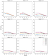 |
Fig. A.1. Trend lines showing the non-LTE effects for unsaturated lines (−6.0 < Wred, λ = log(W/λ) < −4.9) of Ti II across a range of stellar parameters. All models shown have ξt = 2 km s−1 and at least two lines from Table 1. |
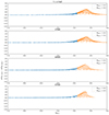 |
Fig. A.2. Difference in abundance for GALAH stars with microturbulences replaced by ξ = 1 and ξ = 2 kms−1 for Ti I. |
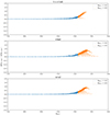 |
Fig. A.3. Difference in abundance for GALAH stars with microturbulences replaced by ξ = 1 and ξ = 2 kms−1 for Ti II. |
All Tables
All Figures
|
Fig. 1. Kiel diagrams showing the values of Teff and log g at which the non-LTE calculations were performed with PySME, as well as the selected GALAH stars for different metallicity ranges. |
| In the text | |
|
Fig. 2. Trend lines showing the non-LTE effects for unsaturated lines (Wred, λ = log(W/λ) < −4.9) of Ti I across a range of stellar parameters. All models shown have ξt = 2 km s−1 and at least two lines from Table 1. |
| In the text | |
|
Fig. 3. Non-LTE abundance correction for A(Ti)Ti I and A(Ti)Ti II, averaged over lines, for the GALAH sample across the Kiel diagram. |
| In the text | |
|
Fig. 4. Non-LTE abundance correction for A(Ti)Ti I and A(Ti)Ti II, averaged over lines, as a function of Teff for the GALAH sample. The trends for dwarfs and giants are shown as solid and dashed lines, respectively, using bins of ΔTeff = ±75 K and limited to bins containing at least 30 stars. The colour gradient represents the number of stars per pixel. |
| In the text | |
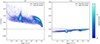 |
Fig. 5. As in Fig. 4, but with a bin size of Δlog g = ±0.1. |
| In the text | |
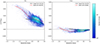 |
Fig. 6. As in Fig. 4, but with a bin size of Δ[Fe/H] = ±0.1. |
| In the text | |
|
Fig. 7. Trend lines showing the non-LTE effects for unsaturated lines (Wred, λ = log(W/λ) < −4.9) of Ti I across five benchmark stars: the Sun (5773, 4.44, 0.00, 1.0), Arcturus (4286, 1.64, −0.53, 1.3), HD84937 (6356, 4.06, −2.06, 1.2), HD140283 (5792, 3.65, −2.36, 1.3), and HD122563 (4636, 1.40, −2.50, 1.8) with parameters of Teff, log g, [Fe/H], and ξt, respectively. |
| In the text | |
|
Fig. 8. Ionisation imbalance, ΔI−II, of titanium at various metallicities in LTE (left) and non-LTE (right) for giants (upper) and dwarfs (lower) from the GALAH sample. The colour gradient and trend lines are the same as in Fig. 6. |
| In the text | |
|
Fig. 9. Ionisation imbalance, ΔI−II, of titanium in metal-poor dwarfs and subgiants from the Keck sample (Sneden et al. 2023) in both LTE and non-LTE for the lines shown in Table 2. Trend lines are the same as in Fig. 6. |
| In the text | |
|
Fig. 10. Run of [Ti/Fe] versus [Fe/H] in LTE (left) and non-LTE (right) from Ti I (upper) and Ti II (lower) for the GALAH sample. Trend lines are the same as in Fig. 6. |
| In the text | |
|
Fig. 11. Star-by-star scatter for dwarfs (left) and giants (right) for different lines of Ti I (upper) and Ti II (lower) from the GALAH sample. The colour gradient and the trend lines are the same as in Fig. 6. |
| In the text | |
|
Fig. 12. Trend of [Ti/Fe] versus [Fe/H] in LTE and non-LTE from Ti I and Ti II. Based on the binning from Fig. 10 for the GALAH sample, averaged over dwarfs and giants. |
| In the text | |
|
Fig. A.1. Trend lines showing the non-LTE effects for unsaturated lines (−6.0 < Wred, λ = log(W/λ) < −4.9) of Ti II across a range of stellar parameters. All models shown have ξt = 2 km s−1 and at least two lines from Table 1. |
| In the text | |
|
Fig. A.2. Difference in abundance for GALAH stars with microturbulences replaced by ξ = 1 and ξ = 2 kms−1 for Ti I. |
| In the text | |
|
Fig. A.3. Difference in abundance for GALAH stars with microturbulences replaced by ξ = 1 and ξ = 2 kms−1 for Ti II. |
| In the text | |
Current usage metrics show cumulative count of Article Views (full-text article views including HTML views, PDF and ePub downloads, according to the available data) and Abstracts Views on Vision4Press platform.
Data correspond to usage on the plateform after 2015. The current usage metrics is available 48-96 hours after online publication and is updated daily on week days.
Initial download of the metrics may take a while.