


| Issue |
A&A
Volume 711, July 2026
|
|
|---|---|---|
| Article Number | A163 | |
| Number of page(s) | 23 | |
| Section | Numerical methods and codes | |
| DOI | https://doi.org/10.1051/0004-6361/202558713 | |
| Published online | 14 July 2026 | |
A fast tree algorithm for the multicomponent coagulation equation
1
Astronomical Science Program, The Graduate University for Advanced Studies (SOKENDAI),
2-21-1 Osawa, Mitaka,
Tokyo
181-8588,
Japan
2
National Astronomical Observatory of Japan,
2-21-1 Osawa, Mitaka,
Tokyo
181-8588,
Japan
★ Corresponding author: This email address is being protected from spambots. You need JavaScript enabled to view it.
Received:
21
December
2025
Accepted:
14
May
2026
Abstract
Context. Dust properties, such as mass, porosity, electric charge, and chemical composition, impact planet formation directly. Understanding the time evolution of dust distribution across multiple properties requires numerical computation. However, the available ways to calculate the multicomponent coagulation-fragmentation equation are highly time-consuming.
Aims. We present a fast and accurate tree algorithm for calculating the multicomponent coagulation equation. We assumed that similar pairs of colliding aggregates reproduce similar outcomes and that the ratio of dust properties in logarithmic space provides the similarity as a “distance”. These assumptions enabled us to apply the tree algorithm, which groups distant bins and calculates averaged interactions, to coagulation. The algorithm reduces the computational complexity from 𝒪(N2d) to 𝒪(dNd log N), considering N bins per d components.
Methods. We tested the tree algorithm by comparing it with the conventional direct method for cases where analytic solutions are known. We measured the dependencies of the wall-clock time, the L2 error in the distribution, and the relative error of the total mass on d, N, the critical opening angle (θc), and the maximum dust distribution width after coagulation (kc).
Results. The algorithm was found to calculate coagulation consistently. For d = 1, the tree method is faster than the direct method for only a specific range of parameters. For d = 2, however, the tree method is faster for all parameter regions surveyed, speeding the calculation up by tens to one hundred times. Increasing N and decreasing θc or kc made it slower and more accurate. Additionally, using a small kc produces worse outcomes than when using a large kc, suggesting that limiting kc is unnecessary.
Conclusions. The fast tree algorithm for the coagulation equation will allow us to evolve the multicomponent dust distribution, such as in mass-porosity space, in protoplanetary disks, ultimately revising planet formation models.
Key words: methods: numerical / planets and satellites: formation / protoplanetary disks / dust, extinction
© The Authors 2026
 Open Access article, published by EDP Sciences, under the terms of the Creative Commons Attribution License (https://creativecommons.org/licenses/by/4.0), which permits unrestricted use, distribution, and reproduction in any medium, provided the original work is properly cited.
This article is published in open access under the Subscribe to Open model. This email address is being protected from spambots. You need JavaScript enabled to view it. to support open access publication.
1 Introduction
Multiple characteristics of a dust aggregate other than mass, including porosity, electrical charge, and chemical composition, are highlighted in planet formation. Planets form in protoplanetary disks through the collisional growth of micron-size dust grains (e.g., Safronov 1972; Hayashi 1981). Planet formation theory has a major problem, as the coagulation of dust particles is hindered by several barriers: radial drift (Adachi et al. 1976; Weidenschilling 1977), bouncing (e.g., Zsom et al. 2010, 2011; Windmark et al. 2012), electrostatic repulsion (Okuzumi 2009; Okuzumi et al. 2011; Akimkin et al. 2020), fragmentation (e.g., Blum & Wurm 2008), and erosion (e.g., Krijt et al. 2015). Recent findings of exoplanets (e.g., Winn & Fabrycky 2015), comets, and asteroids, which are remnants of planetesimals (e.g., A’Hearn 2011), and the existence of our eight planets clearly require that these barriers were overcome. While several mechanisms have been proposed to overcome these barriers, such as the streaming instability (Johansen et al. 2007), one group of the proposed mechanisms is dust microphysics arising from properties other than mass. Porous dust aggregates follow gas flow more closely, weakening the radial drift barrier (Okuzumi et al. 2012; Kataoka et al. 2013a,b). The electric charge of dust aggregates can either stop or promote coagulation since aggregates with the same sign of charge repel each other (Okuzumi 2009; Okuzumi et al. 2011), while those with different signs attract each other (Steinpilz et al. 2020; Teiser et al. 2025). Chemical composition is also key to understanding planet formation, as it can characterize disk environments and determine the elemental and isotopic ratios of planets, asteroids, and comets as the final product (e.g., Öberg et al. 2023). Further understanding of dust aggregates with multiple characteristics, or multicomponent dust aggregates, through theoretical, simulation, observational, and laboratory-experimental perspectives will surely refine the current view of planet formation.
Although numerical coagulation simulations of multicomponent dust aggregates are in high demand, conventional methods are highly time-consuming. The simple, direct method of discretizing the multidimensional distribution of aggregate properties (e.g., mass and volume) and calculating by summation has a computational complexity represented by 𝒪(N2d), where d is the number of components and N is the number of bins per component. The direct method is widely used when only mass is considered (e.g., Stammler & Birnstiel 2022), but it is too costly when other dust characteristics are taken into account. Schemes that utilize the conservation form of the equation (e.g., Ma et al. 2002; Gunawan et al. 2004; Liu et al. 2019; Lombart & Laibe 2021; Laibe & Lombart 2022; Lombart et al. 2022, 2024), cannot handle basic aggregate parameters that do not conserve easily (e.g., volume). Some other fast multicomponent coagulation schemes developed in different fields (e.g., Matveev et al. 2016; Smirnov et al. 2016; Dyachenko et al. 2025) assume a linear gridding for the dust properties and cannot be applied to planet formation, where the scale ranges from micron-size to kilometer-size and logarithmic gridding is required. The methods that average the dust distribution, such as methods of moments (Hulburt & Katz 1964; Estrada & Cuzzi 2008; Estrada et al. 2022), volume-averaging methods (Okuzumi et al. 2012; Kataoka et al. 2013a), and mono-disperse models (e.g., Stepinski & Valageas 1996; Michoulier et al. 2024), cannot be used for situations where the complete information on the multidimensional dust parameter distribution is important. For example, we cannot judge whether a planet on the high-mass end of the distribution forms when tracking just the average of the mass distribution. Even if we tracked the mass distribution carefully but averaged the porosity distribution, it would not be accurate since it is known that bouncing and fragmentation are affected by porosity (e.g., Blum & Wurm 2000; Güttler et al. 2010; Shimaki & Arakawa 2012, 2021; Planes et al. 2021; Oshiro et al. 2025). This implies that a coagulation calculation with a full two-dimensional distribution is required to understand these interactions. Monte Carlo methods require many particles to achieve sufficient accuracy, making them slower than direct methods by orders of magnitude (Drążkowska et al. 2014). Therefore, to fully simulate planet formation and verify the numerical results from various methods, a new algorithm is needed to solve the coagulation of multicomponent dust aggregates.
Here, we present a novel 𝒪(dNd log N) multicomponent coagulation tree algorithm inspired by the tree algorithm in N-body gravity simulations. The tree method for N-body gravity simulations groups together the gravitational force from particles far away and reduces the number of interactions from 𝒪(N2) to 𝒪(N log N) (e.g., Barnes & Hut 1986). A tree data structure represents the geometry or closeness of particles, as the algorithm’s name suggests. We applied this tree method to the coagulation. Our tree algorithm for coagulation assumes that two similar pairs of colliding aggregates result in a similar outcome and that the ratio of dust parameters, such as mass and volume, in logarithmic space is a “distance” (Fig. 1b). With this, we can impose a tree structure on the dust property distribution bins (Fig. 1a). The tree structure holds data of the average dust parameter and the sum of the number density for each grouped bin. The algorithm groups bins far away using the tree and the opening angle criteria (Fig. 1b), and it computes coagulation using the grouped bins (Fig. 1c). By introducing this algorithm, we can reduce the number of interactions and computational complexity from 𝒪(N2d) to 𝒪(dNd log N) (see Section 3.4). This tree method can be used with logarithmic axes and does not assume the conservation of dust properties upon coagulation. Thus, our tree method can be applied to planet formation simulations, such as porosity evolution in protoplanetary disks.
This paper is organized as follows. In Section 2, we review the basic equation – the Smoluchowski coagulation equation (SCE) – and its numerical calculations to provide context. In Section 3, we explain the details of the tree algorithm proposed in our work. In Section 4, we explain the numerical experiment conditions for comparing the tree method and the direct method, which uses simple kernels for which analytic solutions are known. In Section 5, we show the results on how numerical parameters affect calculation speed and numerical accuracy. In Section 6, we discuss our results, techniques for a faster and more accurate scheme, and applications to planet formation. We summarize in Section 7.
 |
Fig. 1 Diagram of tree algorithm for one-component Smoluchowski coagulation calculations. (a) The dust property (here, mass) distribution is discretized into bins, and the bitree corresponds to the hierarchical grouping of the bins. (b) The tree algorithm assumes that the dust parameter space is a virtual metric space, where a distance is defined. To calculate coagulation using the tree, the algorithm first fixes one of the colliding dust aggregates, I-dust, and iterates through the other dust aggregate, II-dust, using the tree. For each level of grouping, the distance between the average of the II-dust bin and the I-dust bin D, the length of the grouped bin L, and the ratio of these two values θ are calculated. (c) The algorithm computes the coagulation (Eq. (34)) using the averaged II-dust bin with the largest bin width under the condition of θ < θc. |
2 Background: The Smoluchowski coagulation equation and its numerical methods
In this section, we review the governing equation for dust coagulation: the SCE and its numerical methods. In Section 2.1, we first cover the one-component version of the equation, where only mass is considered, and in Section 2.2, we review the numerical methods to calculate the one-component equation. In Section 2.3, we cover the multicomponent version, and in Section 2.4, we review the numerical method for the multicomponent equation. In Section 2.5, we explain the conventional and simple direct method, a method that is the basis of our tree method, for the one-component equation. Finally, in Section 2.6, we extend the direct method to the multicomponent equation.
2.1 The one-component Smoluchowski coagulation equation
First, we introduce the coagulation equation of one-component dust aggregates, which have mass as their sole characteristic. The coagulation can be expressed using the following one-component continuous SCE (von Smoluchowski 1916; Müller 1928; Schumann 1940; Safronov 1972):
![Mathematical equation: $\[\begin{aligned}\frac{\partial n(t, m)}{\partial t}= & \frac{1}{2} \int_0^m \mathrm{~d} m^{\prime} R\left(m^{\prime}, m-m^{\prime}\right) n\left(t, m^{\prime}\right) n\left(t, m-m^{\prime}\right) \\& -n(t, m) \int_0^{\infty} \mathrm{d} m^{\prime} R\left(m, m^{\prime}\right) n\left(t, m^{\prime}\right).\end{aligned}\]$](/articles/aa/full_html/2026/07/aa58713-25/aa58713-25-eq1.png) (1)
(1)
If the particle mass can be assumed to be integral multiples of a unit mass (m0), the mass distribution n(m) can be expressed with a discrete distribution (ni), where i is the index corresponding to the mass m = m0i. For the discrete mass distribution, the following one-component discrete SCE is used (von Smoluchowski 1916; Ohtsuki et al. 1990):
![Mathematical equation: $\[\begin{aligned}\frac{\mathrm{d} n_i(t)}{\mathrm{d} t}= & \frac{1}{2} \sum_{j=1}^{i-1} R(i-j, j) n_{i-j}(t) n_j(t) \\& -n_i(t) \sum_{j=1}^{\infty} R(i, j) n_j(t).\end{aligned}\]$](/articles/aa/full_html/2026/07/aa58713-25/aa58713-25-eq2.png) (2)
(2)
These differential-integro equations describe the time evolution of the dust mass distribution. For the continuous equation (Eq. (1)), n(t, m) dm is the number density of dust aggregates with mass from m to m + dm. For the discrete equation (Eq. (2)), n(t, m) is the number density of dust aggregates with mass m. A kernel R(m, m′) = R(m′, m) is a coagulation frequency between mass m and m′ aggregates. The first term on the right-hand side of the equation increases n(t, m) due to the coagulation of mass m′ and m − m′ dust aggregates. The second term decreases n(t, m) due to the coagulation of mass m′ and m dust aggregates. The existence and uniqueness of the solution to the equation is shown by Melzak (1957).
One of the major differences between the continuous equation and the discrete equation is the existence of dust aggregates with mass smaller than the monomer m = m0. The continuous equation allows infinitesimal dust aggregates, but the discrete one only treats the integer multiples of the monomer. This paper focuses on the continuous version of the equation because the multicomponent analytical solutions only exist for the continuous equation (Section 2.3). Infinitely small dust aggregates are nonphysical and purely mathematical, implying that a discrete equation should be preferred in physical applications. However, the numerical simulations for the continuous equation discretize it, which essentially becomes the same as the original discrete equation. The difference explained above turns into the difference in the minimum mass mmin of the grid (and the maximum mass mmax). This slightly affects the numerical setup, which is detailed in Section 2.5 and 2.6.
The SCE calculates the time evolution of the dust mass distribution at only one spatial point, where the distribution can be assumed to be homogeneous. The equation must be calculated at all spatial grids and implemented with advection-diffusion to consider the nonhomogeneity in dust spatial distribution. This paper focuses on the coagulation at only one point in space.
The SCE is used not only for planet formation but also for the coagulation of giant molecular clouds (Kobayashi et al. 2017), dust coagulation in protostellar collapse (Lebreuilly et al. 2023) and the interstellar medium (Hirashita et al. 2021), polymer synthesis (Ziff 1980), nanoparticles (Zhang 2014), and aerosol dynamics (Seigneur et al. 1986). The SCE is also known as the kinetic rate equation (e.g., Ziff 1980), the kinetic collection equation (e.g., Alfonso et al. 2008), and the population balance equation(e.g., Solsvik & and Jakobsen 2015), especially in fields other than astronomy.
For the one-component continuous SCE (Eq. (1)), the following three analytic solutions corresponding to three main simple kernels are known. The three kernels are constant kernel R(mi, mj) = α (also known as “size-independent kernel” in chemical engineering), additive kernel R(mi, mj) = α(mi + mj) (also known as “size-dependent kernel” in chemical engineering), and multiplicative kernel R(mi, mj) = αmimj. Here, α is a constant. The analytic solution for the constant kernel with the initial condition of n(0, m) = N0/m0 exp(−m/m0) is
![Mathematical equation: $\[\tau(t)=\alpha N_0 t,\]$](/articles/aa/full_html/2026/07/aa58713-25/aa58713-25-eq3.png) (3)
(3)
![Mathematical equation: $\[f(t)=\left(1+\frac{\tau(t)}{2}\right)^{-1},\]$](/articles/aa/full_html/2026/07/aa58713-25/aa58713-25-eq4.png) (4)
(4)
![Mathematical equation: $\[x(m)=\frac{m}{m_0},\]$](/articles/aa/full_html/2026/07/aa58713-25/aa58713-25-eq5.png) (5)
(5)
![Mathematical equation: $\[n(t, m)=\frac{N_0}{m_0} f(t)^2 \exp (-f(t) x)\]$](/articles/aa/full_html/2026/07/aa58713-25/aa58713-25-eq6.png) (6)
(6)
(Müller 1928; Schumann 1940; Scott 1968; Silk & Takahashi 1979). Here, m0 is the total mass in the system (constant), and N0 is the initial total number of particles. The analytic solution for the additive kernel with the initial condition of n(0, m) = N0/m0 exp(−m/m0) is
![Mathematical equation: $\[\tau(t)=\alpha N_0 m_0 t,\]$](/articles/aa/full_html/2026/07/aa58713-25/aa58713-25-eq7.png) (7)
(7)
![Mathematical equation: $\[f(t)=\exp (-\tau(t)),\]$](/articles/aa/full_html/2026/07/aa58713-25/aa58713-25-eq8.png) (8)
(8)
![Mathematical equation: $\[g(t)=1-f(t),\]$](/articles/aa/full_html/2026/07/aa58713-25/aa58713-25-eq9.png) (9)
(9)
![Mathematical equation: $\[x(m)=\frac{m}{m_0},\]$](/articles/aa/full_html/2026/07/aa58713-25/aa58713-25-eq10.png) (10)
(10)
![Mathematical equation: $\[n(t, m)=\frac{N_0}{m_0} \frac{f(t)}{x \sqrt{g(t)}} e^{-(2-f(t)) x} I_1(2 x ~\sqrt{g(t)}),\]$](/articles/aa/full_html/2026/07/aa58713-25/aa58713-25-eq11.png) (11)
(11)
where Iν(x) is the modified Bessel function of the first kind (Safronov 1962; Golovin 1963; Scott 1968; Wetherill 1990). The analytic solution for the multiplicative kernel with the initial condition of n(0, m) = N0/m0 · m0/m exp(−m/m0) = N0/m exp(−m/m0) is
![Mathematical equation: $\[\tau(t)=\alpha N_0 m_0^2 t,\]$](/articles/aa/full_html/2026/07/aa58713-25/aa58713-25-eq12.png) (12)
(12)
![Mathematical equation: $\[T(t)=\left\{\begin{array}{ll}\tau(t) & (\tau \leq 1) \\2 \sqrt{\tau(t)}-1 & (\tau \geq 1)\end{array},\right.\]$](/articles/aa/full_html/2026/07/aa58713-25/aa58713-25-eq13.png) (13)
(13)
![Mathematical equation: $\[x(m)=\frac{m}{m_0},\]$](/articles/aa/full_html/2026/07/aa58713-25/aa58713-25-eq14.png) (14)
(14)
![Mathematical equation: $\[n(t, m)=\frac{N_0}{m_0} \frac{1}{x^2 \tau} e^{-(1+T(t)) x} I_1(2 x \sqrt{\tau})\]$](/articles/aa/full_html/2026/07/aa58713-25/aa58713-25-eq15.png) (15)
(15)
(McLeod 1964; Ernst et al. 1984).
For the analytic solutions for the delta function initial condition and ones for the discrete equation, see Appendix B. The analytic solutions for a linear combination of three main kernels (Spouge 1985) and ones for more complicated initial conditions (Scott 1968) are known, but we do not cover these.
The continuous equation can be rewritten using a double integral as
![Mathematical equation: $\[\begin{aligned}\frac{\partial n(t, m)}{\partial t}=\frac{1}{2} & \iint_0^m \mathrm{~d} m_{\mathrm{I}} \mathrm{d} m_{\mathrm{II}} R\left(m_{\mathrm{I}}, m_{\mathrm{II}}\right) n\left(t, m_{\mathrm{I}}\right) n\left(t, m_{\mathrm{II}}\right) \\& \times \delta\left(m-\left(m_{\mathrm{I}}+m_{\mathrm{II}}\right)\right) \\& -n(t, m) \int_0^{\infty} \mathrm{d} m_{\mathrm{II}} R\left(m, m_{\mathrm{II}}\right) n\left(t, m_{\mathrm{II}}\right),\end{aligned}\]$](/articles/aa/full_html/2026/07/aa58713-25/aa58713-25-eq16.png) (16)
(16)
where δ(x) is the Dirac delta function that satisfies ∫ dxδ(x − x0)f(x) = f(x0). The first term on the right-hand side of the SCE (Eq. (16)) expresses the increase in the I+II-dust (m) from the coagulation of the I-dust (mI) and the II-dust (mII). The second term expresses the decrease in the I-dust (m) from the coagulation of the I-dust (m) and the II-dust (mII). Instead of two loops with m and m′ as in Equation (1), the loops in this equation can be regarded as the loops of I-dust and II-dust that are colliding. The subscripts in the first term are as they are, and for the second term, m should be interpreted as mI in the first term. Moreover, this formulation directly connects to the multicomponent version of the equation, which is explained in Section 2.3, and the discretized form for the numerical calculation, as explained in Section 2.5.
2.2 Review of numerical calculations of the one-component Smoluchowski coagulation equation
Since we do not know the analytic solution for the kernel in planet formation, which is much more complex than the ones shown in Section 2.1, we need to calculate the SCE numerically. The SCE calculation can be grouped mainly into two ways. One of them is deterministic methods, which discretize the dust distribution and solve the equation deterministically. The other group of methods is Monte Carlo methods, which randomly sample the dust distribution and evaluate the integrals. Furthermore, the deterministic methods can be classified into three types: the pair-interaction method, the finite element method (FEM), and the method of moments. Section 2.5 of Lombart & Laibe (2021) reviews these methods comprehensively.
The pair-interaction method discretizes the dust parameter distribution into histograms and integrates by summing up the coagulation of all bin pairs. This method is widely used in many preceding studies of planet formation (e.g., Nakagawa et al. 1981; Dullemond & Dominik 2005; Tanaka et al. 2005; Nomura & Nakagawa 2006; Brauer et al. 2008; Birnstiel et al. 2010; Kobayashi & Tanaka 2021; Stammler & Birnstiel 2022), and we refer to this scheme as the “direct method” hereafter. Even limiting to planet formation, its validity has been well studied by Wetherill (1990); Ohtsuki et al. (1990); Lee (2000); Drążkowska et al. (2014). Our novel “tree method”, which we explain later in Section 3, also uses the same discretization but approximates part of the summation.
The FEM discretizes the dust parameter distribution by referencing a conservative form of the equation. In planet formation, Liu et al. (2019); Lombart & Laibe (2021) proposed the discontinuous Galerkin scheme for coagulation based on the conservative form proposed by Tanaka et al. (1996). When applying these methods with an explicit time integration, the Courant–Friedrichs–Lewy conditions for coagulation should be considered for a valid simulation since these methods use a hyperbolic formulation (Laibe & Lombart 2022). Outside planet formation, the population balance equations, which are variations of SCEs, are widely used with FEM. O’Sullivan & Rigopoulos (2022) gives further reviews on those.
The method of moments discretizes the equation using the moments ![Mathematical equation: $\[M_{k}=\int_{0}^{\infty} X^{k} n(t, X) \mathrm{d} X\]$](/articles/aa/full_html/2026/07/aa58713-25/aa58713-25-eq17.png) of the parameter distribution (Hulburt & Katz 1964; Estrada & Cuzzi 2008). In a broader sense, the mono-disperse model can also be included in the method of moments since it uses the mean mass to rewrite the coagulation. The mono-disperse model is computationally less demanding and fits better if the model needs to be coupled with fluid dynamics or chemical network computation (e.g., Stepinski & Valageas 1996, 1997; Kornet et al. 2001; Ciesla & Cuzzi 2006; Garaud 2007; Johansen et al. 2008; Laibe et al. 2008; Sato et al. 2016; Krijt et al. 2018; Garcia & Gonzalez 2020; Michoulier & Gonzalez 2022; Michoulier et al. 2024). Several methods that extend the mono-disperse model have been developed, such as the two-population model (Birnstiel et al. 2012), the tri-population model (Pfeil et al. 2024), and the batch method (Krijt et al. 2016).
of the parameter distribution (Hulburt & Katz 1964; Estrada & Cuzzi 2008). In a broader sense, the mono-disperse model can also be included in the method of moments since it uses the mean mass to rewrite the coagulation. The mono-disperse model is computationally less demanding and fits better if the model needs to be coupled with fluid dynamics or chemical network computation (e.g., Stepinski & Valageas 1996, 1997; Kornet et al. 2001; Ciesla & Cuzzi 2006; Garaud 2007; Johansen et al. 2008; Laibe et al. 2008; Sato et al. 2016; Krijt et al. 2018; Garcia & Gonzalez 2020; Michoulier & Gonzalez 2022; Michoulier et al. 2024). Several methods that extend the mono-disperse model have been developed, such as the two-population model (Birnstiel et al. 2012), the tri-population model (Pfeil et al. 2024), and the batch method (Krijt et al. 2016).
Monte Carlo methods use random numbers to sample (super-) particles from the distribution. These methods are also used widely in planet formation (e.g., Ormel et al. 2007; Zsom & Dullemond 2008; Zsom et al. 2011; Drążkowska et al. 2013; Krijt et al. 2015; Beutel et al. 2024; Vaikundaraman et al. 2025; Gurrutxaga et al. 2026). The comparison with the direct method on numerical accuracy and speed was conducted by Drążkowska et al. (2014).
2.3 The multicomponent Smoluchowski coagulation equation
In this section, we extend the SCE into a multicomponent system. The coagulation of dust aggregates with multiple components, or parameters, is expressed by the multicomponent SCE (Ossenkopf 1993; Kostoglou & Konstandopoulos 2001; Okuzumi et al. 2009):
![Mathematical equation: $\[\begin{aligned}\frac{\partial n(t, \boldsymbol{X})}{\partial t}= & \frac{1}{2} \int \mathrm{d} \boldsymbol{X}_{\mathrm{I}} \mathrm{d} \boldsymbol{X}_{\mathrm{II}} R\left(\boldsymbol{X}_{\mathrm{I}}, \boldsymbol{X}_{\mathrm{II}}\right) n\left(t, \boldsymbol{X}_{\mathrm{I}}\right) n\left(t, \boldsymbol{X}_{\mathrm{II}}\right) \\& \times \delta\left(\boldsymbol{X}-\boldsymbol{X}_{\mathrm{I}+\mathrm{II}}\left(\boldsymbol{X}_{\mathrm{I}}, \boldsymbol{X}_{\mathrm{II}}\right)\right) \\& -n(t, \boldsymbol{X}) \int \mathrm{d} \boldsymbol{X}_{\mathrm{II}} R\left(\boldsymbol{X}, \boldsymbol{X}_{\mathrm{II}}\right) n\left(t, \boldsymbol{X}_{\mathrm{II}}\right),\end{aligned}\]$](/articles/aa/full_html/2026/07/aa58713-25/aa58713-25-eq18.png) (17)
(17)
where X = (X(1), X(2), . . . , X(d)) is the dust aggregate parameter vector with d components. The multidimensional Dirac delta function δ(X, X′) satisfies ∫ dXδ(X − X0) f(X) = f(X0). XI+II (XI, XII) is a function of XI and XII that returns the dust parameter after the coagulation of the two dust aggregates. This formulation is a natural extension of the one-component coagulation equation (Eq. (16)). The variables subscripted with I and II correspond to single-dashed and double-dashed variables in the preceding studies. Here, instead of “single-dashed-dust” or “double-dashed-bin”, we use the terminology of “I-dust” or “II-bins” for simplicity.
For example, to calculate porosity distribution evolution as in Kostoglou & Konstandopoulos (2001); Okuzumi et al. (2009), one would use mass and volume as the dust aggregate parameter X = (X(1), X(2)) = (m, v), and the two-component coagulation equation is expressed as
![Mathematical equation: $\[\begin{aligned}\frac{\partial n(t, m, v)}{\partial t}=\frac{1}{2} & \iiint \int_0^{\infty} \mathrm{d} m_{\mathrm{I}} \mathrm{d} v_{\mathrm{I}} \mathrm{d} m_{\mathrm{II}} \mathrm{d} v_{\mathrm{II}} \\& \times \delta\left(m-\left(m_{\mathrm{I}}+m_{\mathrm{II}}\right)\right) \delta\left(v-v_{\mathrm{III}}\left(m_{\mathrm{I}}, v_{\mathrm{I}}; m_{\mathrm{II}}, v_{\mathrm{II}}\right)\right) \\& \times R\left(m_{\mathrm{I}}, v_{\mathrm{I}}; m_{\mathrm{II}}, v_{\mathrm{II}}\right) n\left(t, m_{\mathrm{I}}, v_{\mathrm{I}}\right) n\left(t, m_{\mathrm{II}}, v_{\mathrm{II}}\right) \\- & n(t, m, v) \int\int_0^{\infty} \mathrm{d} m_{\mathrm{II}} \mathrm{d} v_{\mathrm{II}} \\& \times R\left(m, v; m_{\mathrm{II}}, v_{\mathrm{II}}\right) n\left(t, m_{\mathrm{II}}, v_{\mathrm{II}}\right).\end{aligned}\]$](/articles/aa/full_html/2026/07/aa58713-25/aa58713-25-eq19.png) (18)
(18)
Here, vI+II (mI, vI; mII, vII) is a function that returns the volume after coagulation with void creation and compression included. The maximum of the integration interval in the first term is extended to infinity since the compression may reduce the volume.
One of the challenges with the multicomponent SCE is that it is generally XI+II ≠ XI + XII, which we call the “nonconservative dust property”. Taking dust porosity evolution as an example, dust undergoes fractal growth and compression, leading to non-conservation of volume: vI+II ≠ vI + vII. The nonconservative dust property only refers to the dust parameters after coagulation; other fundamental physical quantities, such as the total mass of the distribution, still conserve even in the SCE with non-conservative dust property.
The multicomponent continuous SCE (Eq. (17)) with conservative dust properties (i.e., XI+II = XI + XII) has analytic solutions, but only for the constant kernel R(XI, XII) = α and the additive kernel R(XI, XII) = α (![Mathematical equation: $\[\sum_{i=1}^{d} X_{\mathrm{I}}^{(i)}+X_{\mathrm{II}}^{(i)}\]$](/articles/aa/full_html/2026/07/aa58713-25/aa58713-25-eq20.png) ), where α is a constant. We only show here the solution for the two-component case, where the dust property vector is X = (m, v), because we only tested the algorithms with one or two components in later sections. The extensions to three or more components are described in the cited works. The analytic solution for the constant kernel with the initial condition of n(0, m, v) = N0/(m0v0)exp(−m/m0 − v/v0) is
), where α is a constant. We only show here the solution for the two-component case, where the dust property vector is X = (m, v), because we only tested the algorithms with one or two components in later sections. The extensions to three or more components are described in the cited works. The analytic solution for the constant kernel with the initial condition of n(0, m, v) = N0/(m0v0)exp(−m/m0 − v/v0) is
![Mathematical equation: $\[\tau(t)=\alpha N_0 t,\]$](/articles/aa/full_html/2026/07/aa58713-25/aa58713-25-eq21.png) (19)
(19)
![Mathematical equation: $\[f(t)=\left(1+\frac{\tau(t)}{2}\right)^{-1},\]$](/articles/aa/full_html/2026/07/aa58713-25/aa58713-25-eq22.png) (20)
(20)
![Mathematical equation: $\[x(m)=\frac{m}{m_0}, \qquad y(v)=\frac{v}{v_0},\]$](/articles/aa/full_html/2026/07/aa58713-25/aa58713-25-eq23.png) (21)
(21)
![Mathematical equation: $\[n(t, m, v)=\frac{N_0}{m_0 v_0} f(t)^2 \exp (-x-y) I_0(2 \sqrt{(1-f(t)) x y})\]$](/articles/aa/full_html/2026/07/aa58713-25/aa58713-25-eq24.png) (22)
(22)
(Lushnikov 1976; Gelbard & Seinfeld 1978; Alexopoulos et al. 2009). The analytic solution for the additive kernel with the initial condition of n(0, m, v) = N0/(m0v0)exp(−m/m0 − v/v0) is
![Mathematical equation: $\[\tau(t)=\alpha N_0\left(m_0+v_0\right) t,\]$](/articles/aa/full_html/2026/07/aa58713-25/aa58713-25-eq25.png) (23)
(23)
![Mathematical equation: $\[f(t)=\exp (-\tau(t)),\]$](/articles/aa/full_html/2026/07/aa58713-25/aa58713-25-eq26.png) (24)
(24)
![Mathematical equation: $\[g(t)=1-f(t),\]$](/articles/aa/full_html/2026/07/aa58713-25/aa58713-25-eq27.png) (25)
(25)
![Mathematical equation: $\[x(m)=\frac{m}{m_0}, \qquad y(v)=\frac{v}{v_0},\]$](/articles/aa/full_html/2026/07/aa58713-25/aa58713-25-eq28.png) (26)
(26)
![Mathematical equation: $\[S(t, m, v)=\sum_{k=0}^{\infty} \frac{\left[x y \frac{m+v}{m_0+v_0} g(t)\right]^k}{(k+1)!(k!)^2},\]$](/articles/aa/full_html/2026/07/aa58713-25/aa58713-25-eq29.png) (27)
(27)
![Mathematical equation: $\[n(t, m, v)=\frac{N_0}{m_0 v_0} f(t) \exp \left(-x-y-\frac{m+v}{m_0+v_0} g(t)\right) S\]$](/articles/aa/full_html/2026/07/aa58713-25/aa58713-25-eq30.png) (28)
(28)
(Fernández-Díaz & Gómez-García 2007; Singh 2021).
2.4 Review of numerical calculations of the multicomponent Smoluchowski coagulation equation
The multicomponent SCE calculation has several computational difficulties. The pair-interaction method is computationally intensive, and the FEM cannot be applied easily to planet formation due to the intrinsic non-conservation of the dust properties. Monte Carlo methods require a large number of particles and substantial computational time to achieve sufficient accuracy. The methods of moments can calculate the multicomponent SCE at a reasonable computational cost and can be applied to planet formation. However, it cannot capture behaviors at the tails of the dust parameter distribution (i.e., the maximum dust size cannot be resolved), and it is invalid if the dust parameter distribution is complex, such as in a bimodal distribution.
The high computational cost of computing the SCE is a universal characteristic. For the pair-interaction method and the FEM, two loops, I and II, are required, leading to a computational complexity of 𝒪(N2d) (Gelbard & Seinfeld 1980). Here, d is the number of parameters or components, and N is the number of bins per parameter. This high computational cost makes it unrealistic to compute the multicomponent (d > 1) SCE directly. This is also true for the FEMs, which can reduce the number of bins N compared to the pair-interaction methods thanks to their high-resolution scheme.
The acceleration of multicomponent SCE calculations has been studied widely. Just as for the one-component SCE computation, it has been studied using FEM, methods of moments, tensor decompositions, Monte Carlo methods, and parallelization.
One approach to accelerate multicomponent SCE calculations is to reduce the number of bins N through (high-order) conservative forms or FEM. The papers that described the discrete Galerkin scheme for the one-component SCE (Liu et al. 2019; Lombart & Laibe 2021; Laibe & Lombart 2022) also discuss the extension to the multicomponent SCE. Ma et al. (2002); Gunawan et al. (2004) proposed high-resolution schemes for the multicomponent population balance equations, a conservative variant of multicomponent SCE. However, applying the conservative forms and FEM to the SCE equations with nonconservative dust properties, such as porosity, is not straightforward (see Section 5.6 of Lombart et al. 2024). Singh et al. (2018) reviews FEM approaches for coagulation.
Another orientation is to rewrite the equation using the moments of the dust parameter distribution. Okuzumi et al. (2012); Kataoka et al. (2013a) averaged the volume of dust aggregates for each mass and reduced the mass-volume multicomponent SCE into the one-component SCE. This model is adopted widely, such as the dust growth in the interstellar medium (Hirashita et al. 2021), and extended to include other physical effects such as evaporation (Estrada et al. 2022). Similar to this, Kostoglou & Konstandopoulos (2001); Kostoglou et al. (2006); Gruy (2011) constructed coagulation models where the fractal dimension of dust aggregates can be written as a time-dependent function, and Otto et al. (2024) constructed a coagulation model that averages porosity for each mass. These “averaging” methods are generally of the methods of moments. The methods of moments are relatively low-cost and valid for planet formation, but they cannot, in principle, derive all the information on the multidimensional dust parameter distribution. For example, the information on the maximum size is required to understand whether a planet can form or not. The effects of dust porosity on fragmentation and bouncing, combined with two or more distinct populations of dust aggregates, can lead to inaccurate calculations. These difficulties imply that a coagulation calculation with a full two-dimensional distribution is required to understand these interactions.
Recent advances in data science have been applied to the multicomponent SCE calculation, creating new approximation methods. Matveev et al. (2016); Smirnov et al. (2016) proposed a method that applies tensor-train decomposition (TT decomposition) (Oseledets 2011), which is a type of tensor decomposition. The SCE in a linear gridding can be rewritten using a lower-triangular convolution (Smirnov et al. 2016), and the convolution can be approximated using TT decomposition (Kazeev et al. 2013). This reduces the computational complexity of multicomponent SCE to 𝒪(d2R4N log N), where R is the maximum TT rank. Another tensor approximation method is the mosaicskeleton approximation (Dyachenko et al. 2025), which can reduce the computational complexity to 𝒪(N(log N)2). However, assuming a linear gridding makes it difficult to apply these methods to planet formation, where scales range from micrometers to kilometers.
Monte Carlo methods for calculating multicomponent SCE are well studied in and out of astronomy (e.g., Laurenzi et al. 2002; Zhao et al. 2010), since they have the advantage that their computational complexity does not increase with the number of components d. However, the fundamental disadvantage of the methods is the same: They require a large number of particles and computational time.
Not only algorithmic improvements but also parallelizations are used to accelerate the SCE computation. As an extension to the TT decomposition method, Zagidullin et al. (2019) parallelized coagulation and advection using MPI and CUDA, resulting in 2–4 times faster. In Monte Carlo methods, Wei & Kruis (2013) used GPU parallelization to accelerate coagulation computation by 10–100 times. Moreover, Xu et al. (2014) implemented the differentially weighted Monte Carlo, and Xu et al. (2015) implemented the Markov jump model to accelerate the calculation further.
2.5 The direct method for the one-component Smoluchowski coagulation equation
Here, we explain the conventional direct method for the one-component SCE, which is the basis of our tree method. The direct method discretizes the dust property distribution and the SCE and calculates the integral by summing up all the bin pairs. We mainly followed Lee (2000); Brauer et al. (2008) for this.
First, the program constructs the bin axes for each dimension of the dust parameters. The axes are in units of the monomer property (i.e., monomer mass m0 = 1, monomer volume v0 = 1). The representative values mi of the first Nbd + 1 bins are on an integer scale from 0 to Nbd. The next Ndec decades with Nbd bins per decade are on the logarithmic grid. The total number of bins is
![Mathematical equation: $\[N=N_{\mathrm{bd}}\left(N_{\mathrm{dec}}+1\right)+1.\]$](/articles/aa/full_html/2026/07/aa58713-25/aa58713-25-eq31.png) (29)
(29)
Combining these constructions into one equation, the representative values of bins are defined by
![Mathematical equation: $\[m_i= \begin{cases}i & \left(i=0,1, \ldots, N_{\mathrm{bd}}\right), \\ N_{\mathrm{bd}} \times 10^{\left(i-N_{\mathrm{bd}}\right) / N_{\mathrm{bd}}} & \left(i=N_{\mathrm{bd}}+1, \ldots, N-1\right).\end{cases}\]$](/articles/aa/full_html/2026/07/aa58713-25/aa58713-25-eq32.png) (30)
(30)
Next, bin boundaries mi–1/2 are defined by the arithmetic average of the representative values of the two neighboring bins
![Mathematical equation: $\[m_{i-1 / 2}=\frac{m_{i-1}+m_i}{2} \quad(i=0,1, \ldots, N).\]$](/articles/aa/full_html/2026/07/aa58713-25/aa58713-25-eq33.png) (31)
(31)
The representative value of the ghost bin before the smallest bin is defined as m−1 = 0 i.e., m−1/2 = 0, and the that of the ghost bin after the largest bin is defined as ![Mathematical equation: $\[m_{N}=r m_{N-1}=m_{N-1}^{2} / m_{N-2}\]$](/articles/aa/full_html/2026/07/aa58713-25/aa58713-25-eq34.png) , assuming a geometric sequence of ratio r = mN–1/mN–2. Lastly, bin widths are defined by the difference between the adjacent boundaries
, assuming a geometric sequence of ratio r = mN–1/mN–2. Lastly, bin widths are defined by the difference between the adjacent boundaries
![Mathematical equation: $\[\Delta m_i=m_{i+1 / 2}-m_{i-1 / 2} \qquad(i=0,1, \ldots, N-1).\]$](/articles/aa/full_html/2026/07/aa58713-25/aa58713-25-eq35.png) (32)
(32)
This “integer-then-logarithmic” grid, first used in Lee (2000), enables the coagulation calculation with a large scale difference from micron-size to kilometer-size with high precision. The former integer part allows for the precise treatment of integer multiples of monomers, especially for the delta function initial conditions or for numerically calculating the discrete version of the equation. The latter logarithmic part treats the large size effectively. Our grid definition is slightly different from the ones in Lee (2000), where they first defined the bin boundary by the integer-then-logarithmic grid and then defined the representative values by the arithmetic average. Our simple tests showed slightly better mass conservation with our axes definition.
Our axis definition also includes the zero-bin, a bin with the representative value of m = 0. This is unnecessary for the discrete equation or the one-component continuous equation, since mass m = 0 added to any other bin has no effect. However, it is necessary for the multicomponent continuous equation, which is described in Section 2.6.
We then discretized the continuous dust number density distribution as
![Mathematical equation: $\[\omega_i(t)=\int_{m_{i-1 / 2}}^{m_{i+1 / 2}} n(t, m) \mathrm{d} m,\]$](/articles/aa/full_html/2026/07/aa58713-25/aa58713-25-eq36.png) (33)
(33)
where mi+1/2 and mi–1/2 are the bin boundaries defined in the Equation (31). Using the defined axis and this discretized distribution, we can discretize the continuous SCE (16) by a simple rectangle method as
![Mathematical equation: $\[\begin{aligned}\frac{\partial \omega_k(t)}{\partial t}= & \frac{1}{2} \sum_{i=0}^k \sum_{j=0}^k K\left(m_i+m_j, m_k\right) R\left(m_i, m_j\right) \omega_i(t) \omega_j(t) \\& -\omega_k(t) \sum_{j=0}^N R\left(m_k, m_j\right) \omega_j(t).\end{aligned}\]$](/articles/aa/full_html/2026/07/aa58713-25/aa58713-25-eq37.png) (34)
(34)
Here, K(mI+II, mk) is an outcome function of a collision. The variables with indices i, j, and k in this discretized equation correspond to the ones with I, II, and no indices in the original continuous equation (Eq. (16)), respectively.
To construct the outcome function K(mI+II, mk), we used a simple first-order scheme. This was first proposed in Kovetz & Olund (1969) and is called the “Podolak algorithm” in astronomy (e.g., Brauer et al. 2008; Stammler & Birnstiel 2022) or the “fixed pivot technique” in chemical engineering (e.g., Kumar & Ramkrishna 1996). Since we used a nonlinear bin axis, the resulting property of coagulation mI+II does not necessarily fall into the representative value of another bin mn but instead falls between mn–1 and mn. This scheme distributes the coagulation term R(mI, mII)n(mI)n(mII) into the two bins. To determine how much of the term should be distributed into each bin, this Podolak algorithm sets the value so that it conserves the total number of particles (i.e., the zeroth moment of the dust distribution) and total mass (i.e., the first moment of the dust distribution) before and after the distribution. Then, the proportion
![Mathematical equation: $\[\epsilon\left(m_{\mathrm{I}+\mathrm{II}}, n\right)=\frac{m_{\mathrm{I}+\mathrm{II}}-m_{n-1}}{m_n-m_{n-1}}\]$](/articles/aa/full_html/2026/07/aa58713-25/aa58713-25-eq38.png) (35)
(35)
of the term is put into bin mn, and 1 − ϵ of the term is put into bin mn–1. Thus, the outcome function K(mI+II, mk) becomes
![Mathematical equation: $\[K\left(m_{\mathrm{I}+\mathrm{II}}, m_k\right)= \begin{cases}\epsilon_m\left(m_{\mathrm{I}+\mathrm{II}}, n\right) & \left(\text { if } m_k=m_n\right), \\ 1-\epsilon_m\left(m_{\mathrm{I}+\mathrm{II}}, n\right) & \left(\text { if } m_k=m_{n-1}\right), \\ 0 & (\text { otherwise }).\end{cases}\]$](/articles/aa/full_html/2026/07/aa58713-25/aa58713-25-eq39.png) (36)
(36)
The indices of the two bins mn–1 and mn of which the dust parameter value after coagulation mI+II falls in between can be calculated by the inverse function of the Equation (30) as
![Mathematical equation: $\[n\left(m_{\mathrm{I}+\mathrm{II}}\right)= \begin{cases}\left\lceil m_{\mathrm{I}+\mathrm{II}}\right\rceil & \left(\text { if } m_{\mathrm{I}+\mathrm{II}} \leq N_{\mathrm{bd}}\right), \\ N_{\mathrm{bd}}+\left\lceil N_{\mathrm{bd}} ~\log _{10} \frac{m_{\mathrm{I}+\mathrm{II}}}{N_{\mathrm{bd}}}\right\rceil & (\text { otherwise }).\end{cases}\]$](/articles/aa/full_html/2026/07/aa58713-25/aa58713-25-eq40.png) (37)
(37)
The pseudocode for the one-component direct method is shown in Appendix A.
The outcome function K only has nonzero values at mn and mn–1, so we can perform all the operations of the first term using the two loops of i and j. The original loop indices for the second term are j and k in the discretized equation, but since the loop range is the same as the first term, we can rename k in the second term as i and do the operations for the second term in the same loop as the first term. This is essentially the same as using two loops, corresponding to the two colliding aggregates of I and II, to calculate both the increase in the I+II-dust and the decrease in the I-dust.
The “empty” nodes and bins, which are bins with zero dust number density, are skipped (continue statement in C++). This reduces computational time considerably in both the direct and tree methods.
At the end of each timestep, the program forces the number density to zero if it is smaller than 10−40. This stabilizes and accelerates the calculation slightly. This is also applied to both the direct method and the tree method.
2.6 The direct method for the multicomponent Smoluchowski coagulation equation
The direct method can be naturally extended to the multicomponent equation. The axis is defined in the same manner for each dust property dimension as the mass axis in the one-component direct method. Using these axes, the d-dimensional array representing the Cartesian dust property grid ![Mathematical equation: $\[\boldsymbol{X}_{\boldsymbol{i}}=\left(X_{i^{(1)}}^{(1)}, X_{i^{(2)}}^{(2)}, \ldots, X_{i^{(d)}}^{(d)}\right)\]$](/articles/aa/full_html/2026/07/aa58713-25/aa58713-25-eq41.png) , where i = (i(1), i(2), . . . , i(d)) is the index vector and X = (X(1), X(2), . . . , X(d)) is the actual dust property corresponding to the index vector, is prepared. In actual implementation, preparing d copies of a one-dimensional axis is enough (i.e., m[mi] and v[vi]).
, where i = (i(1), i(2), . . . , i(d)) is the index vector and X = (X(1), X(2), . . . , X(d)) is the actual dust property corresponding to the index vector, is prepared. In actual implementation, preparing d copies of a one-dimensional axis is enough (i.e., m[mi] and v[vi]).
We used a Cartesian coordinate grid for the performance evaluation in later sections, but different types of grids are available. For example, a two-dimensional polar coordinate (Nandanwar & Kumar 2008) or the X-discretization technique that adopts a diagonal grid (Chauhan et al. 2012) can be used for the two-component SCE.
For the multicomponent continuous equation with an exponentially decreasing initial condition, the small tweak of the zero-bin greatly improves the numerical accuracy. This is because the exponentially decreasing initial condition implies that the infinitesimal aggregates dominate in terms of the number of particles, and the multicomponent distribution can have aggregates with parameters such as (m, v) = (1, 0), (0, 1). The former contributes to diffusing the dust distribution to a larger mass, and the latter contributes to diffusing the dust distribution to a larger volume. These aggregates are nonphysical, but they have a nonnegligible effect of making the numerical solution closer to the mathematical analytic solutions. This zero-bin increases the calculation time by a factor of 5–10, so it should be removed for the physical applications that use the initial condition where everything is a monomer.
The same discretization was applied to the multicomponent equation. The d-dimensional dust parameter distribution is discretized as
![Mathematical equation: $\[\omega_i(t)=\int_{X_{i^{(1)}-1 / 2}^{(1)}}^{X_{i^{(1)}+1 / 2}^{(1)}} \mathrm{d} X^{(1)} \cdots \int_{X_{i^{(d)}-1 / 2}^{(d)}}^{X_{i^{(d)}+1 / 2}^{(d)}} \mathrm{d} X^{(d)} n(t, \boldsymbol{X}),\]$](/articles/aa/full_html/2026/07/aa58713-25/aa58713-25-eq42.png) (38)
(38)
where the total number of bins is
![Mathematical equation: $\[N_{\text {total }}=N^d=\left(N_{\mathrm{bd}}\left(N_{\mathrm{dec}}+1\right)+1\right)^d.\]$](/articles/aa/full_html/2026/07/aa58713-25/aa58713-25-eq43.png) (39)
(39)
The discretized multicomponent continuous SCE is then written as
![Mathematical equation: $\[\begin{aligned}\frac{\partial \omega_k(t)}{\partial t}= & \frac{1}{2} \sum_i \sum_j K\left(\boldsymbol{X}_{\mathrm{I}+\mathrm{II}}\left(\boldsymbol{X}_i, \boldsymbol{X}_j\right), \boldsymbol{X}_k\right) R\left(\boldsymbol{X}_i, \boldsymbol{X}_j\right) \omega_i(t) \omega_j(t) \\& -\omega_k(t) \sum_j R\left(\boldsymbol{X}_k, \boldsymbol{X}_j\right) \omega_j(t).\end{aligned}\]$](/articles/aa/full_html/2026/07/aa58713-25/aa58713-25-eq44.png) (40)
(40)
The Podolak algorithm is also extended to the multicomponent coagulation calculation. The bin that the outcome aggregate falls in (np; Eq. (37)) and the portion of the term (ϵp; Eq. (35)) is calculated for each parameter p using the p-th element of the dust property vector ![Mathematical equation: $\[X_{\mathrm{I}+\mathrm{II}}^{(p)}\]$](/articles/aa/full_html/2026/07/aa58713-25/aa58713-25-eq45.png) . The multicomponent output function K(XI+II, Xk) is defined by the product of output functions for all the axes:
. The multicomponent output function K(XI+II, Xk) is defined by the product of output functions for all the axes:
![Mathematical equation: $\[K\left(\boldsymbol{X}_{\mathrm{I}+\mathrm{II}}, \boldsymbol{X}_{\boldsymbol{k}}\right)=K\left(X_{\mathrm{I}+\mathrm{II}}^{(1)}, X_{k^{(1)}}^{(1)}\right) \cdots K\left(X_{\mathrm{I}+\mathrm{II}}^{(d)}, X_{k^{(d)}}^{(d)}\right).\]$](/articles/aa/full_html/2026/07/aa58713-25/aa58713-25-eq46.png) (41)
(41)
Taking mass-volume space as an example, the pseudocode for the two-component direct method is shown in Appendix A.
More intricate schemes to conserve quantities before and after the distribution can be constructed, such as the modified Podolak algorithm in Brauer et al. (2008) and the three-point framework by Chakraborty & Kumar (2007). Since the difference in choice of these does not affect the major part of our algorithm, we do not cover these.
3 A tree algorithm for the multicomponent Smoluchowski coagulation equation
This section explains our novel tree algorithm for the multicomponent SCE. The key to our tree algorithm is the assumption that property ratios (e.g., mass ratio, volume ratio, etc.) serve as a distance. By defining the distance between bins, we can apply the tree algorithm, which groups bins that are far from the interacting bin partner. Our new coagulation method can reduce the computational cost from 𝒪(N2d) to 𝒪(dNd log N) (see Section 3.4). Our method can also consistently and easily handle the non-conservative coagulation for the first time.
This section is organized as follows. Section 3.1 reviews the concept of the tree algorithm in N-body simulations. Section 3.2 introduces our tree algorithm for the SCE, and Section 3.3 explains it in detail. Section 3.4 describes the strengths and limitations of the tree algorithm.
3.1 Key concept of the tree algorithm in N-body simulations
Before explaining our tree method for SCE, we briefly explain the original tree algorithm in N-body simulations (Barnes & Hut 1986). The simple N-body direct method calculates all the (gravitational) interactions between the N particles. The number of these interactions is the number of all combinations of the particles receiving the force (i-particles) and the particles exerting the force (j-particles), so the computational complexity becomes 𝒪(N2). The N-body Tree Algorithm groups j-particles far away from the i-particle, whose forces are smaller. This reduces the number of interactions and the computational complexity to 𝒪(N log N). A tree data structure, used to group particles, stores the geometric proximity data of the particles. The oct-tree (if 3D), or quad-tree (if 2D), recursively divides the particles into groups and the space into cells, until the cell only contains one particle.
The N-body tree algorithm consists of two parts: tree construction and force iteration using the tree. The tree is constructed by recursively partitioning real space into octo-cells, with half the length for each dimension. The partitioning repeats until there is only one particle in the cell. This tree construction is taken every timestep, every several timesteps, or only during initialization and adjusted every timestep, depending on the extent of optimizations.
After the tree is constructed, the program calculates the gravitational interaction between the particles. The i-particle (receiving the force) is iterated for all particles, and inside the i-loop, j-particles (giving the force) are iterated recursively, starting from the root of the tree. The force from the j-cell is added to the i-particle if the j-cell is sufficiently resolved when seen from the i-particle. If the j-cell is not sufficiently resolved, forces from each child cell inside the j-cell are recursively calculated.
The tree algorithm uses the opening angle θ to determine whether the j-cell is sufficiently resolved or the j-cell can be grouped. The opening angle is defined as follows:
![Mathematical equation: $\[\theta=\frac{L}{D},\]$](/articles/aa/full_html/2026/07/aa58713-25/aa58713-25-eq47.png) (42)
(42)
where L is the length of the j-cell and D is the distance from the i-particle to the mass center of the j-cell. The resolution is enough if θ < θc, where θc is the critical opening angle.
3.2 Introducing the tree algorithm for the Smoluchowski coagulation equation
Here, we introduce a new coagulation method that groups bins, inspired by the N-body tree algorithm. The grouping is possible when the grouped particles or bins (j) give almost the same interactions to the particle or bin of interest (i). In the case of gravitational interactions, only the relative position of particles affects the interaction. The j-particles close together apply similar gravitational forces to the i-particle, due to the smoothness of the gravitational potential. The hierarchical grouping of j-particles by direction and distance, implemented by the gridded space and the opening angle, thus works well with N-body gravity simulations. In the case of the SCE, the interaction is the coagulation of a pair of bins (I and II in the original equation (Eq. (16)), or i and j in the discretized equation (Eq. (34)), and thus the grouped bins (II or j) must have similar coagulation results against the bin to coagulate (I or i). For example, the coagulation of mass i = 1000 and j = 1 aggregates can be practically treated the same as that of mass i = 1000 and j = 2 aggregates.
To convert this idea into a mathematical expression, we assumed that the ratio of dust properties (i.e., mass ratio, volume ratio) of colliding aggregates is a virtual distance (Fig. 1b and Eq. (47)). This essential assumption enables the application of the tree method to coagulation calculation.
The assumption of the distance raises two problems. First, as this assumption only validates the definition of the distance and does not validate the grouping of j-bins far from the i-bin, the feasibility of validating the bin grouping needs to be determined. Second, the valid type of dust property other than mass needs to be determined.
To discuss the validation of the grouping of bins far away, we need to introduce here the major difference between N-body simulations and coagulation calculations: the outcome k-bin. For gravity, only i and j-particles are affected by the interaction between i and j-particles, but for coagulation, k-bins are also affected by the coagulation of i and j-bins. For this additional effect, we need to consider how the grouping of j-bins affects k-bins. Specifically, we need to consider which k-bin is increased and by how much. Another thing to consider in the multicomponent SCE is that it is difficult to analytically calculate the j from k and i. For example, calculating the inverse function of Equation (15) in Okuzumi et al. (2012), a nonlinear model that calculates the volume after coagulation vk from i and j, is difficult. A conservative law for the porosity in this model has not been determined either. This hinders the use of some conservative quantities as a dust parameter other than volume or porosity. This complication also forces the loop indices to be i and j, not k.
The grouping of the j-bins far away in the tree algorithm for the SCE is justified by using the logarithmic grid for the basic dust properties. Let us consider how the grouping of j-bins affects the selection of the k-bin, using mass as a first example. This validation is only important in the first term of the SCE, which describes the increase in the k-bin due to the coagulation of i and j-dust aggregates. If we use the linear grid for the mass, we cannot group the j-bins because the loop index i is fixed within the loop, and the k-bin, calculated by mi + mj = mk, differs for every j. However, by using the logarithmic grid, we can group the j-bins effectively. Since the logarithmic grid partitions bins more finely in smaller quantity regions, there are more j-bins in j < i that satisfy mk−1/2 ≤ mi + mj < mk+1/2, where i and k are fixed. Inside the i-loop, we can group these j-bins and calculate the coagulation of these pairs at once. For example, the increase in mass in the 1000 bin can be calculated at once by grouping the coagulation of mass mi = 990 and mj = 1 aggregates, that of mass mi = 990 and mj = 2 aggregates, etc. This is graphically illustrated using the positions of matrix elements corresponding to k, where the axes of the matrix are i and j (Fig. 2). The diagonal elements in the matrix for the linear grid become bent for the logarithmic grid. Then, we can group the j-bins where the curve is vertical. The farther the j-bins are from the i-bin, the smaller the differences are and the coarser the grouping can be. This supports hierarchical bin grouping, where more distant bins are grouped coarsely.
If the dust property is conservative, then the same justification as mass can be made. Each of the dust parameters is equivalent, and no dust parameter is mathematically special in the multicomponent coagulation equation. This naturally leads to using the same gridding of the bins and extending the bin grouping to multicomponent. This paper evaluates the algorithms with the equations with the conservative dust properties, so the justification above is sufficient.
For the non-conservative dust properties, the justification needs to be made on a case-by-case basis. For example, the effective volume after the coagulation vI+II can be approximated as vI + vII, as long as the logarithmic axis and appropriate porosity model are used (Fig. 3 middle panel). However, for the value of the porosity itself, we cannot conclude the same because the shape of the outcome function of the porosity (Fig. 3 right panel) differs greatly from that of the mass (Fig. 3 left panel). We can conclude that we need to use extensive variables, such as mass, or almost-extensive variables, such as effective volume, for dust parameters in the tree algorithm.
We note that for the simple one-component SCE with mass as the dust property and the linear grid, the mass conservation allowed us to use k as the loop index. The bin pairs (i, j) that give the same k can be grouped, and this idea leads to the diagonal matrix or tensor decomposition methods for the SCE using the linear grid (Matveev et al. 2016; Smirnov et al. 2016; Dyachenko et al. 2025). However for our matter: the multicomponent SCE in planet formation, we cannot do this because (1) the models for components other than mass (e.g., porosity) are often complex and do not have conservation laws, which forbid the grouping of bins by k (as aforementioned), and (2) planet formation needs a much wider range of scales, essentially requiring the logarithmic grid. Paradoxically, we solved these problems by using the logarithmic grid as above.
After the grouping, we can approximate the integral or summation in both terms of the SCE using the average j-bin value. The direct method used the rectangle method with the fixed bin width to discretize the continuous equation. Here, the tree method uses the rectangle method with an adaptive bin width (i.e., the grouped bins have a larger bin width than the non-grouped ones) to discretize the equation (Fig. 4). The farther the j-bins are from the i-bins, the more aggressively they are grouped. The condition on how much the j-bins are grouped is discussed in the next section, and here we explain what happens after the grouping of the bins. The total number of dust aggregates within the grouped j-bin is
![Mathematical equation: $\[\Omega_j=\sum_{j^{\prime} \in j} \omega_{j^{\prime}}(t),\]$](/articles/aa/full_html/2026/07/aa58713-25/aa58713-25-eq48.png) (43)
(43)
and the average representative value of the grouped j-bin is
![Mathematical equation: $\[\overline{\boldsymbol{X}}_j=\frac{1}{\Omega_j} \sum_{j^{\prime} \in j} \omega_{j^{\prime}}(t) \boldsymbol{X}_{j^{\prime}},\]$](/articles/aa/full_html/2026/07/aa58713-25/aa58713-25-eq49.png) (44)
(44)
where j′ ∈ j denotes all the child nodes within the grouped j-bin. The term Ωj corresponds to the total mass within a cell in the gravitational tree algorithm, and ![Mathematical equation: $\[\overline{\boldsymbol{X}}_{\boldsymbol{j}}\]$](/articles/aa/full_html/2026/07/aa58713-25/aa58713-25-eq50.png) corresponds to the center of mass of the cell, respectively. Using this, we could approximate the first term of the SCE as
corresponds to the center of mass of the cell, respectively. Using this, we could approximate the first term of the SCE as
![Mathematical equation: $\[\begin{gathered}\sum_{\boldsymbol{j}} K\left(\boldsymbol{X}_{\mathrm{I}+\mathrm{II}}\left(\boldsymbol{X}_{\boldsymbol{i}}, \boldsymbol{X}_{\boldsymbol{j}}\right), \boldsymbol{X}_{\boldsymbol{k}}\right) R\left(\boldsymbol{X}_{\boldsymbol{i}}, \boldsymbol{X}_{\boldsymbol{j}}\right) \omega_{\boldsymbol{i}}(t) \omega_{\boldsymbol{j}}(t) \\\approx K\left(\boldsymbol{X}_{\mathrm{I}+\mathrm{II}}\left(\boldsymbol{X}_{\boldsymbol{i}}, \overline{\boldsymbol{X}}_{\boldsymbol{j}}\right), \boldsymbol{X}_{\boldsymbol{k}}\right) R\left(\boldsymbol{X}_{\boldsymbol{i}}, \overline{\boldsymbol{X}}_{\boldsymbol{j}}\right) \omega_{\boldsymbol{i}}(t) \Omega_{\boldsymbol{j}}.\end{gathered}\]$](/articles/aa/full_html/2026/07/aa58713-25/aa58713-25-eq51.png) (45)
(45)
The second term of the SCE, which describes the decrease in the k-bin from the coagulation of k and j-dust aggregates, can be similarly approximated as follows:
![Mathematical equation: $\[\begin{aligned}& -\omega_k(t) \sum_{\boldsymbol{X}_j} R\left(\boldsymbol{X}_k, \boldsymbol{X}_j\right) \omega_j(t) \\\approx & -R\left(\boldsymbol{X}_k, \overline{\boldsymbol{X}}_j\right) \omega_k(t) \Omega_j.\end{aligned}\]$](/articles/aa/full_html/2026/07/aa58713-25/aa58713-25-eq52.png) (46)
(46)
Note that the k-bin here corresponds to the i-bin in the first term in the sense of the non-grouped bin of the colliding pair. In both terms, the j-bin is the virtual bin that is created by bin grouping. For this, we need to be careful about the integral interval. The first term of the SCE only needs to be integrated over j < i. However, this second term needs to remove the dust aggregates from the coagulation with all the aggregates, resulting in an integral over a half-infinite region. This means that we have to group not only j-bins that are smaller than k-bins but also larger ones in the second term.
Introduction of the distance into the dust property space and verification of the bin grouping enables us to apply the tree algorithm to the SCE, similarly to N-body simulations (Fig. 1). The tree was constructed bottom-up recursively by creating nodes with 2d adjacent bins as child nodes. Since the geometry of the bins is fixed, this tree construction only takes place in the initialization. The tree needs to be balanced; i.e., the height must be the same (or only differ by one) for all leaves, or it is inefficient. For each timestep, the coagulation, which corresponds to the force in the N-body, was calculated by looping over all i-bins and looping over j-bins using the tree. If i > j, the addition to the k-bin (the first term in the SCE) and the subtraction from the i-bin (the second term in the SCE) were performed, and if i < j, then only the subtraction from the i-bin (the second term in the SCE) was done. The j-bins or nodes are read-only because updating them increases the computational complexity, going back to 𝒪(N2d).
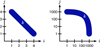 |
Fig. 2 Positions corresponding to k-dust aggregates (outcome of the coagulation) in the (i, j) aggregates (two colliding aggregates) matrix. (Left) When the dust properties are on the linear axes, the k-bin after the coagulation spans diagonally. (Right) When the dust properties are on the logarithmic axes, the k-bin after the coagulation spans along the outwardly convex curve. |
3.3 Detailed explanation of the tree algorithm for the Smoluchowski coagulation equation
This subsection explains the details of the tree algorithm code. We implemented the tree code for the SCE in C++. The pseudocode for the one-component tree method is shown in Appendix B.
In initialization, the program first constructs the bin grid in the same way as the ones in the direct methods previously explained in Sections 2.5 and 2.6. Next, the program instantiates the tree structure. In our code, the tree nodes are represented as structs with the mean dust properties ![Mathematical equation: $\[\overline{\boldsymbol{X}}\]$](/articles/aa/full_html/2026/07/aa58713-25/aa58713-25-eq53.png) , the maximum and minimum dust properties, the dust number density Ω, and pointers to the next node (next) and the first child node (more). The next points to the next sibling node if there is one, or else the aunt-uncle node (the next sibling of the parent node). The grid and bin geometry are the same throughout the simulation, but the mean dust properties and the dust number density must be updated every timestep.
, the maximum and minimum dust properties, the dust number density Ω, and pointers to the next node (next) and the first child node (more). The next points to the next sibling node if there is one, or else the aunt-uncle node (the next sibling of the parent node). The grid and bin geometry are the same throughout the simulation, but the mean dust properties and the dust number density must be updated every timestep.
At every timestep, the program recursively updates the dust property values in the tree and calculates coagulation using the tree. The program recursively updates the values using the depth-first-search iteration. This update costs 𝒪(dNd log N). After the update, the program calculates the coagulation. The program iterates over all the i-bins, then over the j-bins and nodes using the tree. The j-node is assumed to be a singular bin for calculating the coagulation (i.e., the term R(i, j)n(j), the k-bin, and ϵ), with the total mass and the total number density being the sum of the bin values within the node. If the j-node is resolved enough, as defined later, the first term of the SCE is added to the k-bins, and the second term of the SCE is removed from the i-bins. Otherwise, the program iterates over all child nodes of the j-node, treating them as new j-nodes. The j-bins selected using the tree are read-only and are not updated. The “empty” nodes and bins, which are those with zero dust number density, are skipped, similarly to the direct method.
Next, we explain three conditions that determine whether the j-nodes are resolved sufficiently. If all three conditions are satisfied or the j-node is a leaf node (i.e., the bottom-most node), the j-node is adequately resolved, and the coagulation is calculated using that j-node; otherwise, it is not.
The first condition is the opening angle θ, which is also used in the original N-body gravity tree algorithms. We defined the “distance” between two dust property vectors X1 and X2 in the dust property space with logarithmic axes using the L2 norm, i.e.,
![Mathematical equation: $\[\left\|\boldsymbol{X}_1-\boldsymbol{X}_2\right\|=\sqrt{\sum_{p=1}^d\left(\log _{10} X_1^{(p)}-\log _{10} X_2^{(p)}\right)^2}.\]$](/articles/aa/full_html/2026/07/aa58713-25/aa58713-25-eq54.png) (47)
(47)
This distance can be seen as a logarithm of the ratio of dust aggregate properties. The length of the cell L is defined using the distance between the maximum and the minimum of the dust property value within the j-node, and the distance D is defined using the distance between the average property values of the i-bin and j-node (see Fig. 1b). Using these values and the critical opening angle constant θc, we defined it as sufficiently resolved if
![Mathematical equation: $\[\theta=\frac{L}{D}<\theta_c.\]$](/articles/aa/full_html/2026/07/aa58713-25/aa58713-25-eq55.png) (48)
(48)
The smaller θc is, the more resolved the j-node becomes, and the longer and more precise the calculation becomes.
The critical opening angle θc can exceed unity. For example, let us consider a case where the i-bin is the bin next to the maximum of the grouped j-bins and the mass distribution within j-bins is leaning toward the i-bin. The distance D, calculated between the mi and the average value of mj, can become very small. At the same time, the length of the cell L, which is calculated between the maximum and the minimum of mj, can become very large. In this case, the calculated opening angle θ can exceed unity, and the condition for grouping the j-bin in this case can be handled. Even though such a case rarely happens, the critical opening angle θc over unity can be considered.
The second condition is the maximum width of the dust parameter distribution after a coagulation kc. The tree algorithm uses the average value for the j-node, whereas the more precise direct method calculates all the bins within the j-node. This leads to only one value of k in the tree algorithm, compared to multiple values (or a distribution) of k in the direct algorithm. A large variance in the k-dust coming from the j-node distribution can lead to unrealistic numerical diffusion in the tree algorithm. We limit the difference between the virtual maximum and minimum of k to weaken this diffusion. Since calculating the actual maximum and minimum of k is computationally demanding, we assumed a monotonic increase in the dust properties before and after a coagulation. Then, we can use the virtual maximum of k calculated from the maximum of j-node values, and the virtual minimum likewise. The maximum and minimum are obtained for each element of the dust parameter vector. We defined it as resolved enough if
![Mathematical equation: $\[\begin{aligned}\mathrm{(index ~of ~maximum ~virtual} ~k\text{-}\mathrm{dust})\qquad~\\-\mathrm{(index ~of ~minimum ~virtual} ~k\text{-}\mathrm{dust})<k_c,\end{aligned}\]$](/articles/aa/full_html/2026/07/aa58713-25/aa58713-25-eq56.png) (49)
(49)
where kc is the maximum width of the dust parameter distribution after a coagulation. The smaller the kc is, the more resolved the j-node becomes, and the longer and more precise the calculation becomes. Setting kc to be a very large number, such as 1 000 000, is essentially the same as kc = ∞, which means disregarding this second condition.
Note that this kc parameter turns out to be insignificant upon the parameter survey in later sections. This condition was included since we had an intuition that the outcome k, which was not in the original gravitational tree algorithm but is in this tree algorithm for coagulation, might affect the quality of the algorithm, as explained above. To address this question, we put in this parameter kc that can control the quality based on the distribution of the virtual k-bins, and we included this parameter in the explanation.
The third condition is that the i-dust property is not contained within the j-nodes. If at least one of the dust properties of i and j matches, the j-bins cannot be grouped and must be calculated separately. This condition intends to separate the i < j part, where it extends the assumption, and the i > j part, where it does not need the extension of the assumption. The i = j part is also calculated separately. This condition does not have a parameter that can be changed.
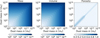 |
Fig. 3 Contour plot of the dust property value after coagulation on the i and j grid. This is the same as Fig. 2, but with concrete numbers. The mass and volume have been normalized using monomer units, i.e., m0 = v0 = 1. (Left) Contour plot of mi + mj. (Middle) Contour plot of effective volume evolution with Okuzumi et al. (2012) model, assuming that the original dust aggregate is compact. (Right) Contour plot of porosity after the coagulation, using the mass and volume from the left and middle panels. |
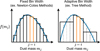 |
Fig. 4 Illustration of numerical integration using the fixed bin width (e.g., Newton-Cotes rectangle method; left) and the adaptive bin width (e.g., our tree method; right). In the adaptive bin width methods, the bin width becomes larger in the farther region, where the virtual distance is the mass ratio of i-dust and j-dust. |
3.4 Strengths and limitations of the tree algorithm for the Smoluchowski coagulation equation
The main advantage of the tree algorithm is its low calculation cost. The overall temporal cost is 𝒪(dNd log N), where d is the number of components and N is the number of bins per component. For example, the tree algorithm for the one-component SCE costs 𝒪(N log N) and for the two-component 𝒪(N2 log N). The breakdown of the time complexity is as follows: the i-dust loop costs 𝒪(Nd), and the j-dust scan using the tree costs as much as the height of the tree, which is 𝒪(log Nd) = 𝒪(d log N) (Knuth 1997). The tree construction occurs only at initialization and thus does not affect the computational speed. Note that this construction also takes 𝒪(dNd log N). The update of the node data, such as total mass, for every time step also takes 𝒪(dNd log N).
A limitation of the tree algorithm is that the bin grouping introduces additional approximation errors. For example, for some of the parameters, the total mass is not conserved. The coagulation equation conserves mass, so its numerical scheme is also desirable to conserve mass. The mass conservation violation of the tree method arises from the breaking of symmetry in the mass transfer from smaller to larger mass bins by coagulation (Fig. 5). The two integrals in the SCE need to be matched during the mass transfer, but the tree algorithm evaluates them independently, leading to the symmetry violation. This is analogous to the breach of Newton’s third law or total momentum conservation in the N-body tree algorithms. This is discussed further in Section 6.3.
4 Methods of algorithm evaluation
This section explains the methods of algorithm evaluation. We measured the speed and errors of the conventional direct method and our tree method, changing the number of components d, the kernel R, the number of bins per component N, the critical opening angle θc, the maximum dust distribution width after a coagulation kc, and the time integration method. The number of components d = 1 corresponds to the mass-only case, and d = 2 corresponds to the mass-and-volume and mass-and-charge cases.
We show the test calculations for two kernels: the constant kernel and the additive kernel. The constant kernel is R(mi, mj) = 1. The additive kernel is R(mi, mj) = (mi + mj)/2 for the one-component cases and R(mi, vi, mj, vj) = (mi + vi + mj + vj)/4 for the two-component cases. The main text omits the multiplicative kernel since it describes gelation, which is beyond our interest, and the analytic solution for the multicomponent multiplicative kernel equation has not been found. The one-component multiplicative kernel is also tested in Appendix B.
The initial condition is set such that analytic solutions have been derived. For the one-component, it is ωi(0) = N0 exp(−mi)Δmi, where the total number of aggregates is normalized to be 1 by ![Mathematical equation: $\[N_{0}^{-1}={\sum}_{i} ~\exp \left(-m_{i}\right) \Delta m_{i}\]$](/articles/aa/full_html/2026/07/aa58713-25/aa58713-25-eq57.png) . For the two-component, it is ωmi,vi(0) = N0 exp(−mi − vi)ΔmiΔvi, where
. For the two-component, it is ωmi,vi(0) = N0 exp(−mi − vi)ΔmiΔvi, where ![Mathematical equation: $\[N_{0}^{-1}={\sum}_{m_{i}, v_{i}} ~\exp \left(-m_{i}-v_{i}\right) \Delta m_{i} \Delta v_{i}\]$](/articles/aa/full_html/2026/07/aa58713-25/aa58713-25-eq58.png) . The analytic solutions for these kernels are shown in Sections 2.1 and 2.3. There are also analytic solutions for the initial condition where the delta function is used. These cases are also tested in Appendix B.
. The analytic solutions for these kernels are shown in Sections 2.1 and 2.3. There are also analytic solutions for the initial condition where the delta function is used. These cases are also tested in Appendix B.
It is rather meaningless to compare results across different kernels, as the important thing is the differences in the various algorithm parameters that affect the results for the same kernel. Testing with different kernels is mainly for algorithm validation, that is, to determine whether the algorithms work for other kernels.
We used the classic fourth-order Runge-Kutta method of coefficients 1/6, 1/3, 1/3, and 1/6 to time integrate Eqs. (34) and (40). We tested two different timesteps: (1) constant time step and (2) adaptive time step. For the constant time step, Table 1 shows the time integration parameters for each kernel. For the adaptive time step, we followed Stammler & Birnstiel (2022); it is calculated such that the dust density ω does not become negative in a first-order Euler scheme considering negative elements of the Δω, with a coefficient of 0.05:
![Mathematical equation: $\[\Delta t_{\text {adaptive }}=0.05 \times \min _i\left|\frac{\omega_i}{\min \left(\Delta \omega_i, 0\right)}\right|.\]$](/articles/aa/full_html/2026/07/aa58713-25/aa58713-25-eq59.png) (50)
(50)
These values of the constant time step and the coefficient for the adaptive time step were set so that the calculation does not crash. The implications of using the explicit time integration methods are discussed further in Section 6.2.
For each of these kernels, we calculated coagulation using the algorithms with parameters in Table 2. We use the number of bins per component N = Nbd(Ndec + 1) + 1 when showing and discussing results, where Nbd is the number of bins in the integer region per component and also the number of bins per decade, and Ndec = 14 is the number of decades per component. The fiducial value for the number of bins per component is N = 241. The fiducial values were chosen to balance the speed and accuracy based on test calculations. As shown in the results, the fiducial kc = 1 000 000 performed better in terms of both speed and accuracy compared with other values of kc. The fiducial θc and N are chosen to balance speed and accuracy.
We measured the following three indices in the algorithm evaluation: (1) wall-clock time (T), (2) L2 error (ε2), and (3) relative error of total mass (ΔM). The wall-clock time (T) is the total execution time the algorithm took to compute. The L2 error (ε2) is the sum of squared differences at the final state (t = tmax) between the analytic distribution m2 na,i and the calculated distribution m2nc,i:
![Mathematical equation: $\[n_{\mathrm{x}, m_i}=\Delta m_i^{-1} \omega_{\mathrm{a}, m_i}\left(t_{\max }\right)\]$](/articles/aa/full_html/2026/07/aa58713-25/aa58713-25-eq60.png) (51)
(51)
![Mathematical equation: $\[n_{\mathrm{X}, m_i, v_i}=\Delta m_i^{-1} \Delta v_i^{-1} \omega_{\mathrm{a}, m_i, v_i}\left(t_{\max }\right)\]$](/articles/aa/full_html/2026/07/aa58713-25/aa58713-25-eq61.png) (52)
(52)
![Mathematical equation: $\[\varepsilon_2=\left\{\begin{array}{l}\sum_{m_i} \Delta m_i m_i^4\left[n_{\mathrm{a}, m_i}-n_{\mathrm{c}, m_i}\right]^2 \\\qquad(d=1), \\\sum_{m_i, v_i} \Delta m_i \Delta v_i m_i^2 v_i^2\left[n_{\mathrm{a}, m_i, v_i}-n_{\mathrm{c}, m_i, v_i}\right]^2 \\\qquad(d=2).\end{array}\right.\]$](/articles/aa/full_html/2026/07/aa58713-25/aa58713-25-eq62.png) (53)
(53)
We used m2n for one-component and mvn for two-component to match the figures of example calculations (i.e., Fig. 6). The relative error of total mass (ΔM) is the absolute difference between the total mass at the final state M(tmax) and that at the initial state M(0), where
![Mathematical equation: $\[M(t)=\left\{\begin{array}{l}\sum_{m_i} \Delta m_i m_i n_{\mathrm{c}}\left(m_i\right), \quad(d=1), \\\sum_{m_i, v_i} \Delta m_i \Delta v_i m_i n_{\mathrm{c}}\left(m_i, v_i\right), \quad(d=2),\end{array}\right.\]$](/articles/aa/full_html/2026/07/aa58713-25/aa58713-25-eq63.png) (54)
(54)
![Mathematical equation: $\[\Delta M=\left|M\left(t_{\max }\right)-M(0)\right|.\]$](/articles/aa/full_html/2026/07/aa58713-25/aa58713-25-eq64.png) (55)
(55)
We used our Mac Studio (2022) for the algorithm evaluation. Its CPU is an Apple M1 Ultra with 20 cores and threads. Since the algorithms are not parallelized, we evaluated them on a single core and thread. There are two types of cores in the CPU: 3.20 GHz and 2.06 GHz, and a simple test using Activity Monitor showed that the evaluation was run on a 3.20 GHz core. The computer has 128 GB of memory. The OS is macOS Ventura 13.5.1.
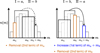 |
Fig. 5 Illustration of symmetry breaking in the tree algorithm for the SCE. The coagulation of mass m = ma and m = mb aggregates was calculated by one operation of the increase with the first term in the equation and two operations of the decrease with the second term. If ma < mb, the increase of ma + mb and the decrease of mb were calculated with one grouping of bins (right panel), and the decrease of ma was calculated with another grouping of bins (left panel). Since these two groupings are different, the total mass exchange is generally nonzero, which means that the total mass is not conserved at the formalization. An operation cannot be performed on the grouped (II or j) bins since it increases the number of operations, diminishing the advantage of the low computational cost of the tree method. |
Timesteps and maximum simulation times used in algorithm evaluation when using a constant time step.
5 Results of algorithm evaluation
This section shows the results for the algorithm evaluation. In Section 5.1, we present examples of the coagulation computations using the direct and tree methods. In Sections 5.2 5.3, 5.4, and 5.5, we show the effects of simulation parameters N, time step, θc, and kc, respectively, on the computational time and accuracy. Finally, in Section 5.6, we demonstrate the trade-off between time and accuracy. Additional tests, for the one-component multiplicative kernel case and the cases with the delta function as the initial condition, are shown in Appendix B.
5.1 Examples of coagulation calculation
Figure 6 shows the time evolution of the one-component (d = 1) dust mass distributions. For all cases, the direct and tree methods are in good overall agreement with the analytic solutions. The main error occurs in the larger tail of the distribution, where the numerical methods produce a heavier tail, leading to a larger maximum dust size. The error is smaller in the constant kernel than in the additive kernel and is also smaller in the large N case than in the fiducial case. This error arises from the numerical diffusion and is common among coagulation calculations (see Drążkowska et al. 2014). The fiducial plots (a) and (d) show that the maximum dust size (i.e., x-intercept) of the tree method is closer to the analytic one than the direct method. This is counterintuitive. It does not mean that the tree method calculates precisely, but the discrepancy is smaller because of another error: the underestimation of maximum dust size due to bin grouping. The error is smaller in the small θc case than in the fiducial case. The underestimation error due to the bin grouping cancels out with the tail overestimation from the numerical diffusion, causing the maximum dust size of the tree method to be closer to the analytic solution than the direct method. These two errors – the overestimation due to the numerical diffusion and the underestimation due to the bin grouping – affect the following error analysis and are discussed further in Section 6.1. The numerical solutions have a small bump at m = Nbdm0 = 16m0 or 40m0, where the gridding changes from linear to logarithmic. The change in the slope at the larger tail of the numerical distribution, especially for the additive kernel, is caused by forcing ω to be zero when ω < 10−40.
Figure 7 shows the two-component (d = 2) dust distributions at the end of the simulation. For all cases, the direct and tree methods are in good overall agreement with the analytic solutions. Since the initial condition is exponentially decreasing n(0, m, v) = N0/(m0v0) exp(−m/m0 − v/v0), infinitesimal dust aggregates with m < 1 (i.e., area left of the m = 100-line in the figure), or v < 1 (i.e., area below the v = 100-line in the figure) exist mathematically. These aggregates disperse the monomer m = v = 1 aggregates to the right or vertically above, which goes against our physical intuition. The sharp tip of the two-dimensional distribution becomes wider and duller in the numerical solutions compared with the analytical solution, which comes from the numerical diffusion. This numerical diffusion is weaker in the large N case than in the fiducial case. In the nonintegrated 2D panels, the difference between the direct method and the tree method is small, but the difference becomes larger to a recognizable degree in the integrated panels. The integrated distribution is similar to the ones in the one-component case, and the two errors can be discussed similarly. The methods in larger N cases have a smaller numerical diffusion error than in the fiducial cases, and the tree method in the smaller θc cases has a smaller underestimation error than in the fiducial cases.
Algorithm parameters explored in the evaluation.
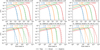 |
Fig. 6 Analytic solutions and results of the numerical calculation of the one-component coagulation equation. The top panels (a), (b), and (c) are for the constant kernel, and the bottom panels (d), (e), and (f) are for the additive kernel. The left panels (a) and (d) were calculated with fiducial parameters Nbd = 16 (i.e., N = 241) and θc = 1; the middle panels (b) and (e) were calculated with a finer grid, Nbd = 40 (i.e., N = 601) and θc = 1; and the right panels (c) and (f) were calculated with a finer bin grouping, Nbd = 16 (i.e., N = 241) and θc = 0.1. In each plot, the sets of lines with four different colors show the snapshots at four different times. In each set, the lines show the tree method with the given θc and kc = 1 000 000 (solid line), the direct method (dashed line), and the analytic solution (dotted line). All numerical results were calculated with adaptive time stepping. |
5.2 Effects of N on speed and accuracy
Figure 8 shows the effect of the number of bins N. The fiducial setting of the time stepping is adaptive, but the N versus T graph for the adaptive time step is hard to understand, so here we show the results for the constant time stepping for N versus T only. Other graphs are calculated using the adaptive time step. The following subsections discuss the figure from top to bottom: N versus T, N versus ε2, and N versus ΔM.
5.2.1 N versus T
The topmost panels of Figure 8 show the wall-clock time T dependence on N. The scaling exponents for this are shown in Table 3. Since the overall trend of the additive kernel is the same as that of the constant kernel, we focus on the constant kernel case.
First, we detail the one-component constant kernel case. The direct method scales as 𝒪(N1.69), which is better than the theoretical estimate of 𝒪(N2). The tree method scales as 𝒪(N1.62) to 𝒪(N1.07) for θc = 0.01 to θc = 10, respectively, which is consistent with the theoretical estimate of 𝒪(N log N), considering adequately large θc case. The tree algorithm with θc = 10 is faster than the direct algorithm at all N, and those with θc = 0.5, 1 are faster than the direct algorithm at N > 200. The tree algorithms with θc = 0.01, 0.1 are slower than the direct algorithm at all N. At the fiducial value N = 241, the tree method with θc = 1 takes 14.7 seconds, while the direct method takes 23.1 seconds to compute; i.e., the tree method was 1.57 times faster.
Next, we continue to the two-component constant kernel case. The direct method scales as 𝒪(N2.80), which is better than the theoretical estimate of 𝒪(N4). The tree method scales as 𝒪(N2.40) to 𝒪(N1.84) for θc = 0.01 to θc = 10, respectively, which is better than the theoretical estimate of 𝒪(N2 log N), considering adequately large θc case. The tree algorithm with parameters explored in this evaluation is faster than the direct algorithm for all N, except the θc = 0.1, N = 61 case. At the fiducial value N = 241, the tree method with θc = 1 takes 12 146.7 seconds, while the direct method takes 72 253.5 seconds to compute; i.e., the tree method was 5.9 times faster. For the large N = 601 case, the tree method with θc = 1 takes 78 762.0 seconds, while the direct method takes 1 080 260 seconds to compute; i.e., the tree method was 13.7 times faster.
For both the one-component and two-component cases, the tree algorithm with a smaller θc, which treats bins more precisely, has worse scaling than the ones with a bigger θc, approaching the scaling of the direct algorithm. The scaling for both methods improves for the two-component than the one-component case, compared with the theoretical estimates. The algorithmic scalings are better than the theoretical estimates of 𝒪(N2d) for the direct algorithm and 𝒪(dNd log N) for the tree algorithm. This can be attributed to the step where the algorithm skips empty bins, as explained in Section 3.3, which considerably reduces computational time.
Scaling exponents for N versus T, for constant time step.
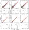 |
Fig. 7 Analytic solutions and results of the numerical calculation of the two-component coagulation equation. The panel layout is the same as Fig. 6, with an additional integrated distribution panel for each case. The upper panel in each subplot (a) through (f) shows the two-dimensional distribution of mvn(m, v), with contour line levels of 10−16, 10−12, 10−8, 10−4, and 1. The bottom panel in each subplot shows the one-dimensional distribution integrated over the secondary component (volume v) to get the distribution of m2 n(m), to match Fig. 6. The panels show the snapshot at the end of the simulation, t = tmax. Three different colors show the three different schemes: the tree method with θc = 1 (blue contour lines), the direct method (red contour lines), and the analytic solution (monochromatic filled contour or grey line). For most cases, the contour lines of the direct method and the tree method overlap in the 2D plot. |
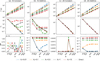 |
Fig. 8 Effect of the number of bins per component N on the wall-clock time T (the top panels), the L2 error ε2 (the middle panels), and the relative error of the total mass ΔM (the bottom panels) for the constant time step. From the left, the panels show the results for the (a) one-component constant kernel, (b) one-component additive kernel, (c) two-component constant kernel, and (d) two-component additive kernel. In each plot, different colors correspond to the direct method, or the different values of θc for the tree methods. All tree method cases were calculated with kc = 1 000 000. For the wall-clock time T, the lines were fit by the least squares method, using the logarithmic values of N and T. |
5.2.2 N versus ε2
First, we detail the L2 error ε2 dependence on N (middle-row panels of Figure 8) for the one-component constant kernel case. The error of the direct method converges to zero as N increases, with scaling of about ε2 ~ 𝒪(N−4). However, for the tree method, the error hits its minimum at some point, depending on the critical opening angle θc. The tree method with a smaller θc, which treats bins more precisely, converges to the direct method: the minimum of the error decreases, and the N at which it occurs increases.
Next, for the one-component additive kernel, the trends for the direct method and the tree method with a smaller θc are the same as the constant kernel, but the trends for the tree method with a larger θc are different. Here, the error for the tree method with a large θc (≥1) stays almost the same for all N, and it makes the error in a small N lower than that of the direct method. We discuss the cause of these strange behaviors of the errors in Section 6.1.
Finally, for the two-component case, all errors behave similarly to those of the one-component direct method. This means that the effect of the critical opening angle θc on the error is limited. Instead, the effect of the numerical diffusion coming from the number of bins N is dominant. This diffusion can be attributed to the sharp tip in the analytic two-dimensional distribution becoming wider and duller in the numerical solutions. The scaling of the error decrease is worse than the one-component case, with scaling of about ε2 ~ 𝒪(N−1). This indicates that the numerical diffusion should be considered more carefully in multicomponent cases than in the one-component case. We note that if the two-component distribution is integrated and compared with the analytical solutions, the same trend as the one-component case, of the error for the tree method not converging to zero, appears.
5.2.3 N versus Δ M
The bottom-most panels of Figure 8 show the relative error of the total mass ΔM dependence on N. In all cases, the error is almost constant for all N’s, with several exceptions. Its value is at the machine epsilon level in the one-component or two-component constant kernel cases with all schemes, and in all kernels with the direct method. In the additive kernel cases, the tree method has a larger error in the total mass, up to 30% for the fiducial parameters. As aforementioned in Section 3.4, the tree method breaks symmetry in the integral, causing this total mass error. Using a smaller value of θc decreases this error, converging to the result of the direct method. The exception of the direct method not conserving mass in the additive kernel at a small N comes from the tail of the mass distribution running over the defined computation mass grid. In the two-component constant kernel case, the tree method with N = 20, 40 behaves strangely.
5.3 Effects of time step choice on speed and accuracy
Figure 9 shows the N-scaling of the wall-clock time T and the wall-clock time per step Tper step for the adaptive time step. The scaling exponents for T are shown in Table 4. The choice of the constant time step or the adaptive time step has almost no effect on the accuracy (i.e., the shape of the distribution, ε2, and ΔM), so these figures are omitted for space.
Compared with the constant time step (topmost panels of Fig. 8), the adaptive time step accelerates the calculation by a factor of tens or even hundreds. The intuitive trend of T (upper panels) increasing with N is the same as with a constant time step, but the details are hard to interpret because the number of steps is adaptively set. The behavior of Tper step (lower panels) is mostly natural, resembling the ones in the constant time step (topmost panels of Fig. 8), except the one-component constant kernel case. In the one-component constant kernel case, the scatter plot of the adaptive time step does not lie on a line and is not monotonically increasing with N. In the two-component additive kernel case, the scatter plot for the total wall-clock time T seems to behave similarly to a quadratic curve. The other two kernels are more natural, with data points on top of the fit lines in both scatter plots.
 |
Fig. 9 Effect of the number of bins per component N on the wall-clock time T (top panels) and the wall-clock time per step Tper step (bottom panels) for the adaptive time step. From the left, the panels show the results for the (a) one-component constant kernel, (b) one-component additive kernel, (c) two-component constant kernel, and (d) two-component additive kernel. In each plot, different colors correspond to the direct method, or the different values of θc for the tree methods. The tree method was calculated with kc = 1 000 000. The lines were fit by the least squares method, using the logarithmic values of N and T. |
Scaling exponents for N versus T, for adaptive time step.
5.4 Effects of θc on speed and accuracy
Figure 10 shows the effect of the critical opening angle θc for the constant time step. The following subsections discuss the figure from top to bottom: θc versus T, θc versus ε2, and θc versus Δ M.
5.4.1 θc versus T
The topmost panels of Figure 10 show the wall-clock time T dependence on the critical opening angle θc. Overall, from small θc to large θc, the time for the tree algorithm increases, then at θc ≈ 0.05, it reaches a maximum (i.e., the computation speed hits a minimum), and finally it decreases and converges to a finite value. The wall-clock time at a small θc = 0.01 does not depend on kc. The time maximum at θc ≈ 0.05 is larger for the one-component than the two-component and also for a smaller kc than a larger kc. Finally, the time at a large θc is almost a constant at θc ≳ 5, and it decreases as kc increases. For the one-component, the tree method is faster than the direct method only when both criteria are sufficiently large, i.e., θc ≳ 0.5 and kc = 1 000 000. For the two-component, the tree method is faster than the direct method across most of the explored parameters.
5.4.2 θc versus ε2
First, we explain the L2 error ε2 dependence on the critical opening angle θc (middle-row panels of Figure 10) for the one-component constant kernel case. There is a clear trend that a large θc makes the tree algorithm less accurate, which is consistent with the theoretical prediction. First, at θc ≲ 0.5, which groups bins finely, the tree method maintains an error equivalent to that of the direct method. Then, at θc ≈ 1, the error increases sharply. Finally, at θc ≳ 5, which groups bins coarsely, the error becomes almost constant. The increase in the error at θc ≈ 1 is larger for a large kc, and a small kc = 1 removes the increase, making it constant for all θc.
Next, for the one-component additive kernel, there is an additional error minimum at θc = 0.5. This minimum makes it more accurate than the direct method at this point. For a large kc, the error sharply increases at θc ≈ 1, making it less accurate than the direct method, but for a small kc = 1, it maintains its low error. As a result, the L2 error becomes smaller as θc becomes larger for the additive kernel with kc = 1, which is against the theoretical estimate.
Finally, for the two-component cases, the L2 error stays nearly the same for any value of θc, paying attention to the y-scale. This means that the critical opening angle θc has a small effect compared with the number of bins N. This is consistent with the results for the N versus ε2 graph (The middle-row panels of Fig. 8). The error of the tree method converges to the value of the direct method at a small θc. In the two-component constant kernel case, the tree method with large θc and kc yields a smaller error than the direct method, which is not straightforward to explain.
 |
Fig. 10 Effect of the critical opening angle θc on the wall-clock time T (the top panels), the L2 error ε2 (the middle panels), and the relative error of the total mass ΔM (the bottom panels) for the constant time step. From the left, the panels show the results for the (a) one-component constant kernel, (b) one-component additive kernel, (c) two-component constant kernel, and (d) two-component additive kernel. Since the critical opening angle θc only affects the tree method, the results for the direct method are shown using a horizontal dotted black line. In each plot, different colors correspond to the different values of kc for the tree methods. All methods were calculated with N = 241. |
5.4.3 θc versus Δ M
The bottom-most panels of Figure 10 show the relative error of the total mass ΔM dependence on the critical opening angle θc. As explained in Section 5.2.3, all schemes maintain the machine epsilon level of the error for the constant kernel cases, and the direct method maintains it for all cases. For the additive kernel cases, similar to the L2 error ε2, the ΔM error increases as θc increases. The increase only happens at θc ≲ 1 and is constant at θc ≳ 1. A large kc increases the error, but its effect is small. For the two-component case, the ΔM error is larger than in the one-component case, with about several percent to 30%.
5.5 Effects of kc on speed and accuracy
5.5.1 kc versus T
From the topmost panels of Figure 10, a larger value of kc, which coarsely treats bins, decreases the time for all cases. This is consistent with the theoretical prediction. The decrease only occurs for θc ≳ 0.1, where the bin grouping takes effect.
5.5.2 kc versus ε2
From the middle-row panels of Figure 10, a larger value of kc increases the L2 error ε2 for the one-component case at a large θc. This is consistent with the theoretical prediction. For the two-component case, the effect of kc is subtle.
5.5.3 kc versus Δ M
For the constant kernel cases, since all schemes conserve the total mass, kc does not affect this error. For the additive kernel cases, a larger value of kc increases the ΔM error (bottom-most panels of Fig. 10). This is consistent with the theoretical prediction.
5.6 Trade-off between speed and accuracy
Figure 11 shows the trade-off between the wall-clock time T and the L2 error ε2, with constant N. A point in the bottom-left part of the figure represents an algorithm parameter that is both time-efficient and accurate; a point in the top-right part represents the opposite. The tree algorithm becomes slower and more accurate by making θc and kc smaller. We can see that for the one-component, the tree algorithm is faster than the direct method for large values of θc and kc. For the two-component, the tree algorithm outperforms the direct algorithm at most of the parameter values. The tree algorithm with a larger kc can be faster and more accurate than those with a smaller kc.
Figure 12 shows the trade-off between the wall-clock time T and the L2 error ε2, with constant kc. Especially for the two-component cases, both algorithms have a scaling law where, as N increases, the time increases and the error decreases. To achieve a desirable error (i.e., to make the point go left of a vertical line in the figure), sufficiently large N and θc are required. The implications for the physical applications are discussed in Section 6.1.
 |
Fig. 11 Comparison of the L2 error ε2 versus wall-clock time T with N = 241. Each point in a line corresponds to different values of θc and kc. From the left, the panels show the results for the (a) one-component constant kernel, (b) one-component additive kernel, (c) two-component constant kernel, and (d) two-component additive kernel. The parameter can be considered good if the point is located lower (faster) and further to the left (more accurate). |
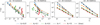 |
Fig. 12 Same as Fig. 11, but for a constant kc = 1 000 000. Each point in a line corresponds to different values of N, where the most time-consuming and most accurate one (top-left) is N = 40 × (14 + 1) + 1 = 601 and the fastest and least accurate one (bottom-right) is N = 4 × (14 + 1) + 1 = 61. |
6 Discussion
6.1 Interpretation of results
The results suggest that our tree method is suitable for the SCE with two or more components. Through parameter search of the algorithm, we find that in the one-component case, the tree algorithm is faster than the direct algorithm for a specific range of parameters. Furthermore, in the two-component case, the tree algorithm outperforms the direct algorithm in all parameter regions surveyed.
Out of these regions, a sufficiently large value of kc = 1 000 000 performed better in both time and accuracy than those with smaller values of kc (Fig. 11). This means that the condition (2) (kc) for the bin grouping, explained in Section 3.3, is unnecessary and can be removed.
Similarly, a large value of θc performed better in both time and accuracy compared with those with a smaller value of θc, especially in the two-component cases. As we discuss later, this is because in the two-component case, the numerical diffusion coming from the insufficient number of bins N is dominant, and the effect of the bin grouping is obscured. This means that the tree method is especially effective in multicomponent coagulation.
We can decide which values of parameters N and θc to use by balancing speed and accuracy based on performance evaluations. A comprehensive study including comparison with the Monte Carlo method by Drążkowska et al. (2014) suggested Nbd = 20 to Nbd = 40, which corresponds to N = 301 to N = 601, to achieve sufficient accuracy. Comparing this with Fig. 12, we can infer that the best tree algorithm parameters are N = 601 and a small value of θc, such as θc = 0.1 for the one-component. Although the bin grouping in the tree algorithm increases the error, it has the advantage of enabling the SCE calculation with two or more components by speeding it up.
One major problem found in the performance evaluation is the high numerical diffusion in the two-component coagulation. This diffusion is common to both the direct and tree methods, as seen in exemplary figures (Fig. 7). This caused a slow convergence in the N versus ε2 figure (middle-row panels in Fig. 8). We have concluded that, to calculate the multicomponent dust coagulation in protoplanetary disks accurately, higher-order schemes are necessary. A promising candidate for a higher-order scheme is to change the algorithm that distributes the mass transfer between the bins from the Podolak algorithm to the extended cell-averaging technique (ECAT) (Kostoglou 2007; Chaudhury et al. 2013). The ECAT is essentially a higher-order Podolak algorithm that additionally considers the second-order moment of a distribution. However, the current ECAT does not consider mass transfer exceeding 15 digits, a machine epsilon of the double-precision float. Such a modification is necessary to make it applicable to planet formation. To make the tree method for the multicomponent coagulation valid for use in planet formation, further investigations, including comparisons with Monte Carlo methods and performance evaluations with physical kernels, are necessary.
The L2 error ε2 of the tree method shows behaviors that are hard to understand. One of them is the response to the number of bins N in the one-component case (middle-row panels of Fig. 8). First, for the constant kernel, the direct method and the tree method with a small θc converge to zero as N increases. The tree method with a large θc hits an error minimum at some N and stays constant from there. For the additive kernel, the direct method and the tree method with a small θc behave the same as the constant kernel, but the tree method with a large θc has an almost-constant error for all N. Another strange behavior is the error’s response to the critical opening angle θc for the additive kernel (Fig. 10). There is a local minimum at θc ≈ 0.5, and here, the error of the tree method is lower than that of the direct method.
The strange behaviors of the L2 error ε2 can be understood through the balance of two error origins: (1) the overestimation of the maximum dust size caused by the numerical diffusion, and (2) the underestimation of the peak size and the maximum dust size by the tree method when θc is large. Let us compare the left panels (fiducial cases) and the middle-column panels (large N cases) of Fig. 6. The former plot exhibits greater numerical diffusion, or the overestimation of the maximum dust size, than the latter. Additionally, the tree method with a larger θc (left panels of Fig. 6) underestimates the peak and the maximum dust size compared with the direct method or the tree method with a smaller θc (right panels of Fig. 6). The underestimation is prominent in the additive kernel. These two numerical effects can cancel each other out, resulting in the tree method performing better than the direct method coincidentally. The point at which this occurs corresponds to the θc for which the tree method has a better accuracy than the direct method in Fig. 10. This might also be a cause for the tree method with a large θc having an almost-constant error for the additive kernel (Fig. 10). Next, due to the numerical diffusion, the tail of the final dust distribution for the additive kernel exceeds the maximum mass bin calculated m = Nbd × 1014. This leads to a large ΔM error at small N (Fig. 8). This also makes the error of the tree method with a large θc smaller than that of the direct method in small N for the additive kernel.
The dependence of the wall-clock time T on the critical opening angle θc is also hard to understand. The local maximum of time at θc ≈ 0.5 (topmost panels in Fig. 10) does not appear for the tree method in N-body gravity simulations (see Hernquist 1987). A smaller value of the kc leads to a larger value at the local maximum, suggesting that the interaction of the grouping criteria kc and θc is important for interpretation. The overhead of the tree method might have caused this.
Our tree method does not exactly conserve the total mass for a specific range of parameters and kernels (e.g., bottom-most panels in Fig. 8). This drawback is analogous to the non-conservation of total momentum in the N-body gravity tree algorithm. The non-conservation comes from the asymmetry in calculating the pairwise interactions. In the N-body tree algorithm, the gravitational force from the i1-particle to the j-particle is grouped with the i2-particle to the j-particle if i1 and i2 are close together. However, the gravitational force from the j-particle to the i1-particle is calculated independently from the force from the j-particle to the i2-particle. This is the asymmetry in calculating the interaction, and it causes the total momentum to be non-conserved. The asymmetry also exists in our tree method for coagulation calculation (Fig. 5), and it analogously causes the total mass to be non-conserved. However, for N-body gravity simulations, a tree algorithm that conserves the total momentum has been developed (Dehnen 2000). This is achieved by using the Taylor expansion in Cartesian coordinates. Developing a similar variant for the SCE tree algorithm is a future issue.
For the one-component constant kernel, the tree method conserves mass. We suppose that the integration of the coagulation term over the distribution for the constant kernel coincidentally matches exactly the rectangle integration method (Fig. 5). This can probably be rephrased as saying that in the constant kernel, higher-order terms of the Taylor expansion of the coagulation term are negligible.
6.2 Time integration of the Smoluchowski coagulation equation
We used the explicit classical fourth-order Runge-Kutta method for the time integration. The coagulation-fragmentation equation in planet formation is known to be stiff, and implicit integration has been used widely (see Brauer et al. 2008; Stammler & Birnstiel 2022). However, the extension from one-component to multicomponent enlarges the Jacobian matrix size from N2 to N2d, where N is the number of bins per component and d is the number of components. Calculating such a large matrix is practically impossible, lowering the superiority of implicit time integrations for multicomponent equations. This Jacobian is also time-varying, which disallows matrix decomposition methods. To overcome these problems, we had to use explicit time integration. However, it actually turned out to be better than the implicit ones. First noted by Rafikov et al. (2020), although the implicit time integrations speed up the calculation by allowing larger time steps, realistic simulations require a moderately small time step to achieve a sufficiently small error. This drops the widely known advantage of the implicit methods being fast and stable, making them comparable to explicit methods. Therefore, we suggest solving the coagulation-fragmentation equations with explicit time-integration methods, even for the one-component and especially for the multicomponent.
We have tested using the constant time step and the adaptive time step in the performance evaluation. The results suggest that using the adaptive one is better, since it is faster while having the same accuracy. Alternative ways of calculating the adaptive time steps, such as the Runge–Kutta–Fehlberg method (RKF45) and the Cash–Karp method, might perform better, but these are future issues.
There should be a restriction on the maximum time step for the pairwise method with explicit time integration, since a time step too large causes the calculation to crash. Related time step restrictions, such as the CFL condition for the hyperbolic, conservative form of the SCE with explicit time integration (Laibe & Lombart 2022), have been investigated. However, the CFL condition cannot be directly applied to our formulation because our formulation is not hyperbolic. A derivation of the corresponding time step restriction is an important topic for future work.
6.3 Variants of tree algorithm for the Smoluchowski coagulation equation
Several variations of our tree method can be hinted at. First, we only tested using the simplest numerical integration: the rectangle rule of Newton-Cotes methods. Other sophisticated methods, such as Simpson’s rule or power-law interpolations within bins (Lee 2000), should perform better. This is analogous to implementing the multipole expansion in the tree method for N-body gravity simulations (e.g., Greengard & Rokhlin 1987; Capuzzo-Dolcetta & Miocchi 1998; Cheng et al. 1999; Dehnen 2014). Different definitions of the “distance” in dust coagulation, such as using the L∞ norm instead of the L2 norm, may be used. More subtle optimizations, such as using arrays instead of structs with pointers, or caching values, may perform better.
In this work, we focused on coagulation, but the tree method can, in principle, also be applied to fragmentation. The difference between coagulation and fragmentation lies in the number of bins for the collision outcome. In coagulation, only the bin of mass mi + mj increases, whereas in fragmentation, an assumed fragmentation mass distribution is used to increase the bins of outcomes. This additional operation on bins requires extra time, but assuming a self-similar distribution can decrease it to a reasonable time (Rafikov et al. 2020).
A fast algorithm for coagulation and fragmentation, such as our tree method, benefits many astrophysical studies on dust distribution evolution. Multiple components of dust particles, including porosity, electric charge, chemical composition, and temperature, have been studied recently. These studies often assume empirical and approximate models, such as the mono-disperse models (e.g., Michoulier et al. 2024). These models need to be checked with more accurate coagulation-fragmentation models, fitting the necessary parameters (e.g., Pfeil et al. 2024). Our tree algorithm enables the multicomponent distribution-aware dust coagulation calculation with accurate physical models in a spatial-1D (radius) disk, such as DustPy (Stammler & Birnstiel 2022), for the first time. With this algorithm, how multicomponent dust aggregates grow in protoplanetary disks can be studied accurately, providing insights into refined planet formation models.
7 Summary and conclusion
Multicomponent dust aggregates play an important role in planet formation. The multicomponent coagulation (and fragmentation) calculation is necessary, but its high computational cost is an obstacle. We developed a novel tree algorithm for the multicomponent coagulation calculation inspired by the tree algorithm used in N-body gravity simulations. It assumes that similar pairs of colliding aggregates reproduce similar outcomes if they have similar properties and that the dust property ratio gives the similarity as a “distance”. Denoting the two colliding aggregates as i-dust and j-dust, this assumption enabled us to group the adjacent j-dust bins “far away” from the i-dust bin. The bin grouping is performed according to the critical opening angle θc and the maximum dust distribution width kc. Grouping the bins allows the algorithm to calculate coagulation faster than the conventional direct method. We tested this approach by comparing it with the analytic solutions and the direct method. We assessed the dependence of the wall-clock time T, the L2 error in the distribution function ε2, and the relative error of the total mass conservation ΔM on the number of components d = 1, 2; kernels R; number of bins N; critical opening angle θc; maximum dust distribution width after a coagulation kc; and time integration method. Our conclusions are as follows:
For the one-component equation, our tree method is faster than the direct method when the critical opening angle θc is sufficiently large. For the two-component equation, our tree method is systematically faster than the direct method across all parameter regions surveyed. For example, the tree method was 5.9 times faster than the direct method for the fiducial parameters and 13.7 times faster for the larger N = 601 case;
The primary numerical parameter of the tree method is the critical opening angle θc, which effectively controls the trade-off between computational cost and accuracy. A larger θc yields a faster computation but larger errors. We find that kc is not important, and removing it makes the calculation faster while maintaining the same accuracy;
The tree method reproduces the overall behavior well, with the main deviations arising from (1) an overestimation of the maximum dust size caused by the numerical diffusion, which is also present in the direct method, and (2) a slight underestimation of the peak and the maximum dust size due to bin grouping. The first error can be reduced by making N larger, and the second error can be reduced by making θc smaller;
For a specific range of parameters and kernels, the tree method does not exactly conserve the total mass. However, this deviation can be reduced by adopting a smaller critical opening angle θc.
Altogether, our tree method is a first step toward a complete coagulation calculation for multicomponent dust aggregates. In future work, we plan to apply this approach to the time evolution of the dust porosity distribution in protoplanetary disks while incorporating various phenomena. Developing a fully mass-conserving higher-order formulation of the tree method is an important subject for future work. We have also noted a possible variant of the tree method for fragmentation schemes applicable to planet formation.
Code availability
The code is available upon reasonable request.
Acknowledgements
The authors would like to deeply appreciate the anonymous referee for comments, which greatly helped in improving the manuscript. The authors would also like to appreciate Shota Notsu, Kazunari Iwasaki, and Yuki Kambara for fruitful discussions. The authors would also like to appreciate Sota Arakawa, Shubham Bhardwaj, Ryotaro Chiba, Uma Gorti, Shu-ichiro Inutsuka, Yuichiro Ishida, Hiroshi Kobayashi, Eiichiro Kokubo, Naoto Maki, Hiroki Nagakura, Hideko Nomura, Keiji Ohtsuki, Satoshi Okuzumi, Chen Peng-Fei, Shota Sato, Sin-iti Sirono, Hidekazu Tanaka, Kei Tanaka, and Yuki Yoshida for valuable comments. T.K.W. acknowledges support through the NAOJ Junior Fellow Program. This work was supported by JSPS KAKENHI Grant Number JP22K03680. This work was partially supported by Overseas Travel Fund for Students (2025) of Astronomical Science Program, The Graduate University for Advanced Studies, SOKENDAI. The authors acknowledge Grammarly’s help in improving only the writing. Software: GNU Parallel (Tange 2026), NumPy (Harris et al. 2020), Matplotlib (Hunter 2007), Pandas (The pandas development team 2020), and SciPy (Virtanen et al. 2020).
References
- Adachi, I., Hayashi, C., & Nakazawa, K. 1976, Prog. Theor. Phys., 56, 1756 [CrossRef] [Google Scholar]
- A’Hearn, M. F. 2011, ARA&A, 49, 281 [Google Scholar]
- Akimkin, V. V., Ivlev, A. V., & Caselli, P. 2020, ApJ, 889, 64 [NASA ADS] [CrossRef] [Google Scholar]
- Alexopoulos, A. H., Roussos, A., & Kiparissides, C. 2009, Chem. Eng. Sci., 64, 3260 [Google Scholar]
- Alfonso, L., Raga, G. B., & Baumgardner, D. 2008, Atmos. Chem. Phys., 8, 969 [Google Scholar]
- Barnes, J., & Hut, P. 1986, Nature, 324, 446 [NASA ADS] [CrossRef] [Google Scholar]
- Beutel, M., Dullemond, C. P., & Strzodka, R. 2024, A&A, 684, A2 [NASA ADS] [CrossRef] [EDP Sciences] [Google Scholar]
- Birnstiel, T., Dullemond, C. P., & Brauer, F. 2010, A&A, 513, A79 [NASA ADS] [CrossRef] [EDP Sciences] [Google Scholar]
- Birnstiel, T., Klahr, H., & Ercolano, B. 2012, A&A, 539, A148 [NASA ADS] [CrossRef] [EDP Sciences] [Google Scholar]
- Blum, J., & Wurm, G. 2000, Icarus, 143, 138 [NASA ADS] [CrossRef] [Google Scholar]
- Blum, J., & Wurm, G. 2008, ARA&A, 46, 21 [CrossRef] [Google Scholar]
- Brauer, F., Dullemond, C. P., & Henning, T. 2008, A&A, 480, 859 [NASA ADS] [CrossRef] [EDP Sciences] [Google Scholar]
- Capuzzo-Dolcetta, R., & Miocchi, P. 1998, J. Comput. Phys., 143, 29 [Google Scholar]
- Chakraborty, J., & Kumar, S. 2007, Chem. Eng. Sci., 62, 4112 [Google Scholar]
- Chaudhury, A., Kapadia, A., Prakash, A. V., Barrasso, D., & Ramachandran, R. 2013, Adv. Powder Technol., 24, 962 [Google Scholar]
- Chauhan, S. S., Chiney, A., & Kumar, S. 2012, Chem. Eng. Sci., 70, 135 [Google Scholar]
- Cheng, H., Greengard, L., & Rokhlin, V. 1999, J. Comput. Phys., 155, 468 [Google Scholar]
- Ciesla, F. J., & Cuzzi, J. N. 2006, Icarus, 181, 178 [NASA ADS] [CrossRef] [Google Scholar]
- Dehnen, W. 2000, ApJ, 536, L39 [NASA ADS] [CrossRef] [Google Scholar]
- Dehnen, W. 2014, ComAC, 1, 1 [Google Scholar]
- Drążkowska, J., Windmark, F., & Dullemond, C. P. 2013, A&A, 556, A37 [NASA ADS] [CrossRef] [EDP Sciences] [Google Scholar]
- Drążkowska, J., Windmark, F., & Dullemond, C. P. 2014, A&A, 567, A38 [NASA ADS] [CrossRef] [EDP Sciences] [Google Scholar]
- Dullemond, C. P., & Dominik, C. 2005, A&A, 434, 971 [CrossRef] [EDP Sciences] [Google Scholar]
- Dyachenko, R. R., Matveev, S. A., & Valiakhmetov, B. I. 2025, arXiv e-prints [arXiv:2501.10206] [Google Scholar]
- Ernst, M. H., Ziff, R. M., & Hendriks, E. M. 1984, J. Colloid Interface Sci., 97, 266 [Google Scholar]
- Estrada, P. R., & Cuzzi, J. N. 2008, ApJ, 682, 515 [Google Scholar]
- Estrada, P. R., Cuzzi, J. N., & Umurhan, O. M. 2022, ApJ, 936, 42 [NASA ADS] [CrossRef] [Google Scholar]
- Fernández-Díaz, J. M., & Gómez-García, G. J. 2007, EPL, 78, 56002 [Google Scholar]
- Garaud, P. 2007, ApJ, 671, 2091 [NASA ADS] [CrossRef] [Google Scholar]
- Garcia, A. J., & Gonzalez, J.-F. 2020, MNRAS, 493, 1788 [Google Scholar]
- Gelbard, F. M., & Seinfeld, J. H. 1978, J. Colloid Interface Sci., 63, 472 [Google Scholar]
- Gelbard, F., & Seinfeld, J. H. 1980, J. Colloid Interface Sci., 78, 485 [Google Scholar]
- Golovin, A. M. 1963, Bulletin of the Academy of Sciences of the U.S.S.R., Geophysics Series, 5, 783 [Google Scholar]
- Greengard, L., & Rokhlin, V. 1987, J. Comput. Phys., 73, 325 [NASA ADS] [CrossRef] [Google Scholar]
- Gruy, F. 2011, Colloids Surf. A: Physicochem. Eng. Aspects, 374, 69 [Google Scholar]
- Gunawan, R., Fusman, I., & Braatz, R. D. 2004, AIChE J, 50, 2738 [Google Scholar]
- Gurrutxaga, N., Vaikundaraman, V., & Drazkowska, J. 2026, A&A, 709, A164 [NASA ADS] [CrossRef] [EDP Sciences] [Google Scholar]
- Güttler, C., Blum, J., Zsom, A., Ormel, C. W., & Dullemond, C. P. 2010, A&A, 513, A56 [Google Scholar]
- Harris, C. R., Millman, K. J., van der Walt, S. J., et al. 2020, Nature, 585, 357 [NASA ADS] [CrossRef] [Google Scholar]
- Hayashi, C. 1981, Prog. Theor. Phys. Suppl., 70, 35 [Google Scholar]
- Hernquist, L. 1987, ApJS, 64, 715 [NASA ADS] [CrossRef] [Google Scholar]
- Hirashita, H., Il’in, V. B., Pagani, L., & Lefèvre, C. 2021, MNRAS, 502, 15 [NASA ADS] [CrossRef] [Google Scholar]
- Hulburt, H. M., & Katz, S. 1964, Chem. Eng. Sci., 19, 555 [Google Scholar]
- Hunter, J. D. 2007, CiSE, 9, 90 [Google Scholar]
- Johansen, A., Oishi, J. S., Low, M.-M. M., et al. 2007, Nature, 448, 1022 [NASA ADS] [CrossRef] [Google Scholar]
- Johansen, A., Brauer, F., Dullemond, C., Klahr, H., & Henning, T. 2008, A&A, 486, 597 [NASA ADS] [CrossRef] [EDP Sciences] [Google Scholar]
- Kataoka, A., Tanaka, H., Okuzumi, S., & Wada, K. 2013a, A&A, 557, L4 [NASA ADS] [CrossRef] [EDP Sciences] [Google Scholar]
- Kataoka, A., Tanaka, H., Okuzumi, S., & Wada, K. 2013b, A&A, 554, A4 [NASA ADS] [CrossRef] [EDP Sciences] [Google Scholar]
- Kazeev, V. A., Khoromskij, B. N., & Tyrtyshnikov, E. E. 2013, SIAM J. Sci. Comput., 35, A1511 [Google Scholar]
- Knuth, D. E. 1997, The Art of Computer Programming: Fundamental Algorithms, 1 (Addison-Wesley Professional) [Google Scholar]
- Kobayashi, H., & Tanaka, H. 2021, ApJ, 922, 16 [NASA ADS] [CrossRef] [Google Scholar]
- Kobayashi, M. I., Inutsuka, S.-i., Kobayashi, H., & Hasegawa, K. 2017, ApJ, 836, 175 [NASA ADS] [CrossRef] [Google Scholar]
- Kornet, K., Stepinski, T. F., & Różyczka, M. 2001, A&A, 378, 180 [NASA ADS] [CrossRef] [EDP Sciences] [Google Scholar]
- Kostoglou, M. 2007, J. Colloid Interface Sci., 306, 72 [Google Scholar]
- Kostoglou, M., & Konstandopoulos, A. G. 2001, J. Aerosol Sci., 32, 1399 [Google Scholar]
- Kostoglou, M., Konstandopoulos, A. G., & Friedlander, S. K. 2006, J. Aerosol Sci., 37, 1102 [Google Scholar]
- Kovetz, A., & Olund, B. 1969, J. Atmos. Sci. [Google Scholar]
- Krijt, S., Ormel, C. W., Dominik, C., & Tielens, A. G. G. M. 2015, A&A, 574, A83 [NASA ADS] [CrossRef] [EDP Sciences] [Google Scholar]
- Krijt, S., Ormel, C. W., Dominik, C., & Tielens, A. G. G. M. 2016, A&A, 586, A20 [NASA ADS] [CrossRef] [EDP Sciences] [Google Scholar]
- Krijt, S., Schwarz, K. R., Bergin, E. A., & Ciesla, F. J. 2018, ApJ, 864, 78 [Google Scholar]
- Kumar, S., & Ramkrishna, D. 1996, Chem. Eng. Sci., 51, 1311 [Google Scholar]
- Laibe, G., & Lombart, M. 2022, MNRAS, 510, 5220 [Google Scholar]
- Laibe, G., Gonzalez, J.-F., Fouchet, L., & Maddison, S. T. 2008, A&A, 487, 265 [NASA ADS] [CrossRef] [EDP Sciences] [Google Scholar]
- Laurenzi, I. J., Bartels, J. D., & Diamond, S. L. 2002, J. Comput. Phys., 177, 418 [Google Scholar]
- Lebreuilly, U., Vallucci-Goy, V., Guillet, V., Lombart, M., & Marchand, P. 2023, MNRAS, 518, 3326 [Google Scholar]
- Lee, M. H. 2000, Icarus, 143, 74 [Google Scholar]
- Liu, H., Gröpler, R., & Warnecke, G. 2019, SIAM J. Sci. Comput., 41, B448 [CrossRef] [Google Scholar]
- Lombart, M., & Laibe, G. 2021, MNRAS, 501, 4298 [Google Scholar]
- Lombart, M., Hutchison, M., & Lee, Y.-N. 2022, MNRAS, 517, 2012 [CrossRef] [Google Scholar]
- Lombart, M., Bréhier, C.-E., Hutchison, M., & Lee, Y.-N. 2024, MNRAS, 533, 4410 [CrossRef] [Google Scholar]
- Lushnikov, A. A. 1976, J. Colloid Interface Sci., 54, 94 [Google Scholar]
- Ma, D. L., Tafti, D. K., & Braatz, R. D. 2002, Ind. Eng. Chem. Res., 41, 6217 [Google Scholar]
- Matveev, S. A., Zheltkov, D. A., Tyrtyshnikov, E. E., & Smirnov, A. P. 2016, J. Comput. Phys., 316, 164 [Google Scholar]
- McLeod, J. B. 1964, Proc. Lond. Math. Soc., 3, 445 [Google Scholar]
- Melzak, Z. 1957, Trans. Am. Math. Soc., 85, 547 [CrossRef] [Google Scholar]
- Michoulier, S., & Gonzalez, J.-F. 2022, MNRAS, 517, 3064 [NASA ADS] [CrossRef] [Google Scholar]
- Michoulier, S., Gonzalez, J.-F., & Price, D. J. 2024, A&A, 688, A31 [NASA ADS] [CrossRef] [EDP Sciences] [Google Scholar]
- Müller, H. 1928, Kolloidchem Beih, 27, 223 [Google Scholar]
- Nakagawa, Y., Nakazawa, K., & Hayashi, C. 1981, Icarus, 45, 517 [NASA ADS] [CrossRef] [Google Scholar]
- Nandanwar, M. N., & Kumar, S. 2008, Chem. Eng. Sci., 63, 2198 [Google Scholar]
- Nomura, H., & Nakagawa, Y. 2006, ApJ, 640, 1099 [Google Scholar]
- Öberg, K. I., Facchini, S., & Anderson, D. E. 2023, ARA&A, 61, 287 [Google Scholar]
- Ohtsuki, K., Nakagawa, Y., & Nakazawa, K. 1990, Icarus, 83, 205 [NASA ADS] [CrossRef] [Google Scholar]
- Okuzumi, S. 2009, ApJ, 698, 1122 [Google Scholar]
- Okuzumi, S., Tanaka, H., & Sakagami, M.-a. 2009, ApJ, 707, 1247 [NASA ADS] [CrossRef] [Google Scholar]
- Okuzumi, S., Tanaka, H., Takeuchi, T., & Sakagami, M.-a. 2011, ApJ, 731, 95 [Google Scholar]
- Okuzumi, S., Tanaka, H., Kobayashi, H., & Wada, K. 2012, ApJ, 752, 106 [NASA ADS] [CrossRef] [Google Scholar]
- Ormel, C. W., Spaans, M., & Tielens, A. G. G. M. 2007, A&A, 461, 215 [NASA ADS] [CrossRef] [EDP Sciences] [Google Scholar]
- Oseledets, I. V. 2011, SIAM J. Sci. Comput., 33, 2295 [Google Scholar]
- Oshiro, H., Tatsuuma, M., Okuzumi, S., & Tanaka, H. 2025, ApJ, 983, 75 [Google Scholar]
- Ossenkopf, V. 1993, A&A, 280, 617 [NASA ADS] [Google Scholar]
- O’Sullivan, D., & Rigopoulos, S. 2022, Chem. Eng. Sci., 263, 117925 [Google Scholar]
- Otto, E., Ajalova, A., Bück, A., Tsotsas, E., & Kienle, A. 2024, Ind. Eng. Chem. Res., 63, 17545 [Google Scholar]
- Pfeil, T., Birnstiel, T., & Klahr, H. 2024, A&A, 691, A45 [NASA ADS] [CrossRef] [EDP Sciences] [Google Scholar]
- Planes, M. B., Millán, E. N., Urbassek, H. M., & Bringa, E. M. 2021, MNRAS, 503, 1717 [CrossRef] [Google Scholar]
- Rafikov, R. R., Silsbee, K., & Booth, R. A. 2020, ApJS, 247, 65 [Google Scholar]
- Safronov, V. S. 1962, Dokl. Akad. Nauk SSSR, 147, 64 [Google Scholar]
- Safronov, V. S. 1972, Evolution of the Protoplanetary Cloud and Formation of the Earth and Planets (Israel Program for Scientific Translations, Keter Publishing House) [Google Scholar]
- Sato, T., Okuzumi, S., & Ida, S. 2016, A&A, 589, A15 [NASA ADS] [CrossRef] [EDP Sciences] [Google Scholar]
- Schumann, T. E. W. 1940, Quart. J. Roy. Meteorol. Soc., 66, 195 [Google Scholar]
- Scott, W. T. 1968, J. Atmos. Sci., 25, 54 [Google Scholar]
- Seigneur, C., Hudischewskyj, A. B., Seinfeld, J. H., et al. 1986, Aerosol Sci. Technol., 5, 205 [Google Scholar]
- Shimaki, Y., & Arakawa, M. 2012, Icarus, 221, 310 [NASA ADS] [CrossRef] [Google Scholar]
- Shimaki, Y., & Arakawa, M. 2021, Icarus, 369, 114646 [NASA ADS] [CrossRef] [Google Scholar]
- Silk, J., & Takahashi, T. 1979, ApJ, 229, 242 [NASA ADS] [CrossRef] [Google Scholar]
- Singh, M. 2021, Stud. Appl. Math., 147, 955 [Google Scholar]
- Singh, M., Kaur, G., De Beer, T., & Nopens, I. 2018, Reac. Kinet. Mech. Cat., 123, 385 [Google Scholar]
- Smirnov, A. P., Matveev, S. A., Zheltkov, D. A., & Tyrtyshnikov, E. E. 2016, Proc. Comput. Sci., 80, 2141 [Google Scholar]
- Solsvik, J., & Jakobsen, H. A. 2015, J. Dispers. Sci. Technol., 36, 510 [Google Scholar]
- Spouge, J. L. 1985, J. Phys. A, Math. Gen., 18, 3063 [Google Scholar]
- Stammler, S. M., & Birnstiel, T. 2022, ApJ, 935, 35 [NASA ADS] [CrossRef] [Google Scholar]
- Steinpilz, T., Joeris, K., Jungmann, F., et al. 2020, Nat. Phys., 16, 225 [Google Scholar]
- Stepinski, T. F., & Valageas, P. 1996, A&A, 309, 301 [NASA ADS] [Google Scholar]
- Stepinski, T. F., & Valageas, P. 1997, A&A, 319, 1007 [NASA ADS] [Google Scholar]
- Tanaka, H., Inaba, S., & Nakazawa, K. 1996, Icarus, 123, 450 [Google Scholar]
- Tanaka, H., Himeno, Y., & Ida, S. 2005, ApJ, 625, 414 [NASA ADS] [CrossRef] [Google Scholar]
- Tange, O. 2026, https://doi.org/10.5281/zenodo.18735643 [Google Scholar]
- Teiser, J., Penner, J., Joeris, K., et al. 2025, Nat Astron, 9, 535 [Google Scholar]
- The pandas development team 2020, https://doi.org/10.5281/zenodo.3509134 [Google Scholar]
- Vaikundaraman, V., Gurrutxaga, N., & Drążkowska, J. 2025, arXiv e-prints [arXiv:2507.21239] [Google Scholar]
- Virtanen, P., Gommers, R., Oliphant, T. E., et al. 2020, Nat. Methods, 17, 261 [Google Scholar]
- von Smoluchowski, M. 1916, Z. Phys., 17, 585 [Google Scholar]
- Wei, J., & Kruis, F. E. 2013, J. Comput. Phys., 249, 67 [Google Scholar]
- Weidenschilling, S. J. 1977, MNRAS, 180, 57 [Google Scholar]
- Wetherill, G. W. 1990, Icarus, 88, 336 [NASA ADS] [CrossRef] [Google Scholar]
- Windmark, F., Birnstiel, T., Güttler, C., et al. 2012, A&A, 540, A73 [NASA ADS] [CrossRef] [EDP Sciences] [Google Scholar]
- Winn, J. N., & Fabrycky, D. C. 2015, ARA&A, 53, 409 [NASA ADS] [CrossRef] [Google Scholar]
- Xu, Z., Zhao, H., & Zheng, C. 2014, J. Aerosol Sci., 74, 11 [Google Scholar]
- Xu, Z., Zhao, H., & Zheng, C. 2015, J. Comput. Phys., 281, 844 [Google Scholar]
- Zagidullin, R., Smirnov, A., Matveev, S., & Tyrtyshnikov, E. 2019, in Supercomputing, eds. V. Voevodin & S. Sobolev (Cham: Springer International Publishing), 403 [Google Scholar]
- Zhang, W. 2014, in Nanomaterial: Impacts on Cell Biology and Medicine, eds. D. G. Capco, & Y. Chen (Dordrecht: Springer Netherlands), 19 [Google Scholar]
- Zhao, H., Kruis, F. E., & Zheng, C. 2010, J. Comput. Phys., 229, 6931 [Google Scholar]
- Ziff, R. M. 1980, J. Stat. Phys., 23, 241 [Google Scholar]
- Zsom, A., & Dullemond, C. P. 2008, A&A, 489, 931 [NASA ADS] [CrossRef] [EDP Sciences] [Google Scholar]
- Zsom, A., Ormel, C. W., Güttler, C., Blum, J., & Dullemond, C. P. 2010, A&A, 513, A57 [NASA ADS] [CrossRef] [EDP Sciences] [Google Scholar]
- Zsom, A., Ormel, C. W., Dullemond, C. P., & Henning, T. 2011, A&A, 534, A73 [NASA ADS] [CrossRef] [EDP Sciences] [Google Scholar]
Appendix A Pseudocodes
Here, we show the pseudocode for the one-component direct method 1, the two-component direct method 2, and the one-component tree method 3. The two-component tree method is omitted since it can be naturally composed from the two-component direct method and the one-component tree method.
for all i, j do
if ω[i] < 10−40 ∨ ω[j] < 10−40 then
continue
end if
mI+II ← m[i] + m[j]
k ← n(mI+II) (Eq. (37))
ϵ ← ϵ(mI+II, k) (Eq. (35))
Roo ← R(m[i], m[j]) × ω[i] × ω[j]
Δω[k] ← Δω[k] + 0.5 × Roo × ϵ (first term)
Δω[k − 1] ← Δω[k − 1] + 0.5 × Roo × (1 − ϵ) (first term)
Δω[i] ← Δω[i] − Roo (second term)
end for
for all mi, vi, mj, vj do
if ω[mi, vi] < 10−40 ∨ ω[mj, vj] < 10−40 then
continue
end if
mI+II ← m[mi] + m[mj]
vI+II ← vI+II (m[mi], v[vi], m[mj], v[vj])
mk ← n(mI+II) Eq. (37))
vk ← n(vI+II) (Eq. (37))
ϵm ← ϵ(mI+II, mk) (Eq. (35))
ϵv ← ϵ(vI+II, vk) (Eq. (35))
Roo ← R(m[mi], v[vi], m[mj], v[vj]) × ω[mi, vi] × ω[mj, vj]
Δω[mk, vk] ← Δω[mk, vk] + 0.5 × Roo × ϵmϵv
Δω[mk, vk − 1] ← Δω[mk, vk − 1] + 0.5 × Roo × ϵm(1 − ϵv)
Δω[mk − 1, vk] ← Δω[mk − 1, vk] + 0.5 × Roo × (1 − ϵm) ϵv
Δω[mk − 1, vk − 1] ← Δω[mk − 1, vk − 1] + 0.5 × Roo × (1 − ϵm) (1 − ϵv)
Δω[mi, vi] ← Δω[mi, vi] − Roo
end for
update_tree(root, ω)
for all i do
if ω[i] < 10−40 then
continue
end if
Roo ← R(m[i], m[i]) × ω[i] × ω[i]
k ← n(2 × m[i]) (Eq. (37))
ϵ ← ϵ (2 × m[i], k) (Eq. (35))
Δω[k] ← Δω[k] + 0.5 × Roo × ϵ (first term)
Δω[k − 1] ← Δω[k − 1] + 0.5 × Roo × (1 − ϵ) (first term)
Δω[i] ← Δω[i] − Roo (second term)
j ← root
while j ≠ null do
if j.Ω < 10−40 then
j ← j.next
continue
end if
L ← ∥j.mmax − j.mmin∥ (Eq. (47))
D ← ∥m[i] − j.mavel∥ (Eq. (47))
morecond1 ← (L/D ≥ θc) (Eq. (48))
kmax ← n(m[i] + j.mmax) (Eq. (37))
kmin ← n(m[i] + j.mmin) (Eq. (37))
morecond2 ← (kmax − kmin ≥ kc) (Eq. (49))
morecond3 ← (j.mmin ≤ m[i] ≤ j.mmax)
if !j.is_leaf ∧ (morecond1 ∨ morecond2 ∨ morecond3)
then
j ← j.more
continue
end if
Roo ← R(m[i], j.mave) × ω[i] × j.Ω
Δω[i] ← Δω[i] − Roo (second term)
if m[i] < j.mave then
j ← j.next
continue
end if
mI+II ← m[i] + j.mave
k ← n(mI+II) (Eq. (37))
ϵ ← ϵ(mI+II, k) (Eq. (35))
Δω[k] ← Δω[k] + 0.5 × Roo × ϵ (first term)
Δω[k − 1] ← Δω[k − 1] + 0.5 × Roo × (1 − ϵ) (first term)
j ← j.next
end while
end for
Appendix B Additional tests
Here, additional tests for the three kernels with the one-component discrete SCE, or the one-component continuous SCE with the delta function as the initial condition, are shown. Figure B.1 shows the exemplary results for these cases.
For the one-component discrete SCE (Eq. 2), the following three analytic solutions corresponding to three main simple kernels are known. The three kernels are constant kernel R(mi, mj) = α (also known as “size-independent kernel” in chemical engineering), additive kernel R(mi, mj) = α(mi + mj) (also known as “size-dependent kernel” in chemical engineering), and multiplicative kernel R(mi, mj) = αmimj. Here, α is a constant. The analytic solution for the constant kernel is
![Mathematical equation: $\[n(t, m)=N_0 g(t)^2(1-g(t))^{m-1},\]$](/articles/aa/full_html/2026/07/aa58713-25/aa58713-25-eq65.png) (B.1)
(B.1)
![Mathematical equation: $\[g(t)=\left(1+\frac{\tau(t)}{2}\right)^{-1},\]$](/articles/aa/full_html/2026/07/aa58713-25/aa58713-25-eq66.png) (B.2)
(B.2)
![Mathematical equation: $\[\tau(t)=\alpha N_0 t.\]$](/articles/aa/full_html/2026/07/aa58713-25/aa58713-25-eq67.png) (B.3)
(B.3)
 |
Fig. B.1 Analytic solutions and results of the numerical calculation of the one-component coagulation equation. The top panels (a), (b), and (c) are for the constant kernel; the middle-row panels (d), (e), and (f) are for the additive kernel; and the bottom panels (g), (h), and (i) are for the multiplicative kernel. The left panels (a), (d), and (g) were calculated with fiducial parameters Nbd = 16 (i.e., N = 241) and θc = 1; the middle panels (b), (e), and (h) were calculated with a finer grid, Nbd = 40 (i.e., N = 601) and θc = 1; and the right panels (c), (f), and (i) were calculated with a finer bin grouping, Nbd = 16 (i.e., N = 241) and θc = 0.1. In each plot, the sets of lines with four different colors show the snapshots at four different times. In each set, the lines show the tree method with the given θc and kc = 1000000 (solid line), the direct method (dashed line), and the analytic solution (dotted line). All numerical results were calculated with adaptive time stepping. |
The analytic solution for the additive kernel is
![Mathematical equation: $\[n(t, m)=N_0 \frac{m^{m-1}}{m!} g(t)(1-g(t))^{m-1} e^{-m(1-g(t))},\]$](/articles/aa/full_html/2026/07/aa58713-25/aa58713-25-eq68.png) (B.4)
(B.4)
![Mathematical equation: $\[g(t)=e^{-\tau(t)},\]$](/articles/aa/full_html/2026/07/aa58713-25/aa58713-25-eq69.png) (B.5)
(B.5)
![Mathematical equation: $\[\tau(t)=\alpha N_0 t.\]$](/articles/aa/full_html/2026/07/aa58713-25/aa58713-25-eq70.png) (B.6)
(B.6)
The analytic solution for the multiplicative kernel is
![Mathematical equation: $\[n(t, m)=N_0 \frac{(2 m)^{m-1}}{m!m}\left(\frac{\tau(t)}{2}\right)^{m-1} e^{-m \tau(t)},\]$](/articles/aa/full_html/2026/07/aa58713-25/aa58713-25-eq71.png) (B.7)
(B.7)
![Mathematical equation: $\[\tau(t)=\alpha N_0 t\]$](/articles/aa/full_html/2026/07/aa58713-25/aa58713-25-eq72.png) (B.8)
(B.8)
(Wetherill 1990). The initial condition is n(0, m) = δ(m, 1)N0 for all cases, where
![Mathematical equation: $\[\delta(x)= \begin{cases}1 & \text { if } x=0, \\ 0 & \text { otherwise }\end{cases}\]$](/articles/aa/full_html/2026/07/aa58713-25/aa58713-25-eq73.png) (B.9)
(B.9)
is the Kronecker delta function.
All Tables
Timesteps and maximum simulation times used in algorithm evaluation when using a constant time step.
All Figures
|
Fig. 1 Diagram of tree algorithm for one-component Smoluchowski coagulation calculations. (a) The dust property (here, mass) distribution is discretized into bins, and the bitree corresponds to the hierarchical grouping of the bins. (b) The tree algorithm assumes that the dust parameter space is a virtual metric space, where a distance is defined. To calculate coagulation using the tree, the algorithm first fixes one of the colliding dust aggregates, I-dust, and iterates through the other dust aggregate, II-dust, using the tree. For each level of grouping, the distance between the average of the II-dust bin and the I-dust bin D, the length of the grouped bin L, and the ratio of these two values θ are calculated. (c) The algorithm computes the coagulation (Eq. (34)) using the averaged II-dust bin with the largest bin width under the condition of θ < θc. |
| In the text | |
|
Fig. 2 Positions corresponding to k-dust aggregates (outcome of the coagulation) in the (i, j) aggregates (two colliding aggregates) matrix. (Left) When the dust properties are on the linear axes, the k-bin after the coagulation spans diagonally. (Right) When the dust properties are on the logarithmic axes, the k-bin after the coagulation spans along the outwardly convex curve. |
| In the text | |
|
Fig. 3 Contour plot of the dust property value after coagulation on the i and j grid. This is the same as Fig. 2, but with concrete numbers. The mass and volume have been normalized using monomer units, i.e., m0 = v0 = 1. (Left) Contour plot of mi + mj. (Middle) Contour plot of effective volume evolution with Okuzumi et al. (2012) model, assuming that the original dust aggregate is compact. (Right) Contour plot of porosity after the coagulation, using the mass and volume from the left and middle panels. |
| In the text | |
|
Fig. 4 Illustration of numerical integration using the fixed bin width (e.g., Newton-Cotes rectangle method; left) and the adaptive bin width (e.g., our tree method; right). In the adaptive bin width methods, the bin width becomes larger in the farther region, where the virtual distance is the mass ratio of i-dust and j-dust. |
| In the text | |
|
Fig. 5 Illustration of symmetry breaking in the tree algorithm for the SCE. The coagulation of mass m = ma and m = mb aggregates was calculated by one operation of the increase with the first term in the equation and two operations of the decrease with the second term. If ma < mb, the increase of ma + mb and the decrease of mb were calculated with one grouping of bins (right panel), and the decrease of ma was calculated with another grouping of bins (left panel). Since these two groupings are different, the total mass exchange is generally nonzero, which means that the total mass is not conserved at the formalization. An operation cannot be performed on the grouped (II or j) bins since it increases the number of operations, diminishing the advantage of the low computational cost of the tree method. |
| In the text | |
|
Fig. 6 Analytic solutions and results of the numerical calculation of the one-component coagulation equation. The top panels (a), (b), and (c) are for the constant kernel, and the bottom panels (d), (e), and (f) are for the additive kernel. The left panels (a) and (d) were calculated with fiducial parameters Nbd = 16 (i.e., N = 241) and θc = 1; the middle panels (b) and (e) were calculated with a finer grid, Nbd = 40 (i.e., N = 601) and θc = 1; and the right panels (c) and (f) were calculated with a finer bin grouping, Nbd = 16 (i.e., N = 241) and θc = 0.1. In each plot, the sets of lines with four different colors show the snapshots at four different times. In each set, the lines show the tree method with the given θc and kc = 1 000 000 (solid line), the direct method (dashed line), and the analytic solution (dotted line). All numerical results were calculated with adaptive time stepping. |
| In the text | |
|
Fig. 7 Analytic solutions and results of the numerical calculation of the two-component coagulation equation. The panel layout is the same as Fig. 6, with an additional integrated distribution panel for each case. The upper panel in each subplot (a) through (f) shows the two-dimensional distribution of mvn(m, v), with contour line levels of 10−16, 10−12, 10−8, 10−4, and 1. The bottom panel in each subplot shows the one-dimensional distribution integrated over the secondary component (volume v) to get the distribution of m2 n(m), to match Fig. 6. The panels show the snapshot at the end of the simulation, t = tmax. Three different colors show the three different schemes: the tree method with θc = 1 (blue contour lines), the direct method (red contour lines), and the analytic solution (monochromatic filled contour or grey line). For most cases, the contour lines of the direct method and the tree method overlap in the 2D plot. |
| In the text | |
|
Fig. 8 Effect of the number of bins per component N on the wall-clock time T (the top panels), the L2 error ε2 (the middle panels), and the relative error of the total mass ΔM (the bottom panels) for the constant time step. From the left, the panels show the results for the (a) one-component constant kernel, (b) one-component additive kernel, (c) two-component constant kernel, and (d) two-component additive kernel. In each plot, different colors correspond to the direct method, or the different values of θc for the tree methods. All tree method cases were calculated with kc = 1 000 000. For the wall-clock time T, the lines were fit by the least squares method, using the logarithmic values of N and T. |
| In the text | |
|
Fig. 9 Effect of the number of bins per component N on the wall-clock time T (top panels) and the wall-clock time per step Tper step (bottom panels) for the adaptive time step. From the left, the panels show the results for the (a) one-component constant kernel, (b) one-component additive kernel, (c) two-component constant kernel, and (d) two-component additive kernel. In each plot, different colors correspond to the direct method, or the different values of θc for the tree methods. The tree method was calculated with kc = 1 000 000. The lines were fit by the least squares method, using the logarithmic values of N and T. |
| In the text | |
|
Fig. 10 Effect of the critical opening angle θc on the wall-clock time T (the top panels), the L2 error ε2 (the middle panels), and the relative error of the total mass ΔM (the bottom panels) for the constant time step. From the left, the panels show the results for the (a) one-component constant kernel, (b) one-component additive kernel, (c) two-component constant kernel, and (d) two-component additive kernel. Since the critical opening angle θc only affects the tree method, the results for the direct method are shown using a horizontal dotted black line. In each plot, different colors correspond to the different values of kc for the tree methods. All methods were calculated with N = 241. |
| In the text | |
|
Fig. 11 Comparison of the L2 error ε2 versus wall-clock time T with N = 241. Each point in a line corresponds to different values of θc and kc. From the left, the panels show the results for the (a) one-component constant kernel, (b) one-component additive kernel, (c) two-component constant kernel, and (d) two-component additive kernel. The parameter can be considered good if the point is located lower (faster) and further to the left (more accurate). |
| In the text | |
|
Fig. 12 Same as Fig. 11, but for a constant kc = 1 000 000. Each point in a line corresponds to different values of N, where the most time-consuming and most accurate one (top-left) is N = 40 × (14 + 1) + 1 = 601 and the fastest and least accurate one (bottom-right) is N = 4 × (14 + 1) + 1 = 61. |
| In the text | |
|
Fig. B.1 Analytic solutions and results of the numerical calculation of the one-component coagulation equation. The top panels (a), (b), and (c) are for the constant kernel; the middle-row panels (d), (e), and (f) are for the additive kernel; and the bottom panels (g), (h), and (i) are for the multiplicative kernel. The left panels (a), (d), and (g) were calculated with fiducial parameters Nbd = 16 (i.e., N = 241) and θc = 1; the middle panels (b), (e), and (h) were calculated with a finer grid, Nbd = 40 (i.e., N = 601) and θc = 1; and the right panels (c), (f), and (i) were calculated with a finer bin grouping, Nbd = 16 (i.e., N = 241) and θc = 0.1. In each plot, the sets of lines with four different colors show the snapshots at four different times. In each set, the lines show the tree method with the given θc and kc = 1000000 (solid line), the direct method (dashed line), and the analytic solution (dotted line). All numerical results were calculated with adaptive time stepping. |
| In the text | |
Current usage metrics show cumulative count of Article Views (full-text article views including HTML views, PDF and ePub downloads, according to the available data) and Abstracts Views on Vision4Press platform.
Data correspond to usage on the plateform after 2015. The current usage metrics is available 48-96 hours after online publication and is updated daily on week days.
Initial download of the metrics may take a while.