


| Issue |
A&A
Volume 711, July 2026
|
|
|---|---|---|
| Article Number | A94 | |
| Number of page(s) | 23 | |
| Section | Cosmology (including clusters of galaxies) | |
| DOI | https://doi.org/10.1051/0004-6361/202553802 | |
| Published online | 03 July 2026 | |
Euclid: Field-level inference of primordial non-Gaussianity and cosmic initial conditions★
1
INAF-Osservatorio di Astrofisica e Scienza dello Spazio di Bologna, Via Piero Gobetti 93/3, 40129 Bologna, Italy
2
INFN-Bologna, Via Irnerio 46, 40126 Bologna, Italy
3
Institut d’Astrophysique de Paris, 98bis Boulevard Arago, 75014 Paris, France
4
Oskar Klein Centre for Cosmoparticle Physics, Department of Physics, Stockholm University, Stockholm SE-106 91, Sweden
5
Institut d’Astrophysique de Paris, UMR 7095, CNRS, and Sorbonne Université, 98 bis boulevard Arago, 75014 Paris, France
6
Instituto de Física Teórica UAM-CSIC, Campus de Cantoblanco, 28049 Madrid, Spain
7
CERCA/ISO, Department of Physics, Case Western Reserve University, 10900 Euclid Avenue, Cleveland, OH 44106, USA
8
Dipartimento di Fisica e Scienze della Terra, Università degli Studi di Ferrara, Via Giuseppe Saragat 1, 44122 Ferrara, Italy
9
Istituto Nazionale di Fisica Nucleare, Sezione di Ferrara, Via Giuseppe Saragat 1, 44122 Ferrara, Italy
10
School of Physics and Astronomy, Queen Mary University of London, Mile End Road, London E1 4NS, UK
11
Department of Physics and Astronomy, University of the Western Cape, Bellville, Cape Town, 7535, South Africa
12
Department of Physics, P.O. Box 64, 00014 University of Helsinki, Finland
13
Helsinki Institute of Physics, Gustaf Hällströmin katu 2, University of Helsinki, Helsinki, Finland
14
Dipartimento di Fisica e Astronomia “G. Galilei”, Università di Padova, Via Marzolo 8, 35131 Padova, Italy
15
INFN-Padova, Via Marzolo 8, 35131 Padova, Italy
16
INAF-Osservatorio Astronomico di Padova, Via dell’Osservatorio 5, 35122 Padova, Italy
17
European Space Agency/ESTEC, Keplerlaan 1, 2201 AZ, Noordwijk, The Netherlands
18
Institute Lorentz, Leiden University, Niels Bohrweg 2, 2333 CA, Leiden, The Netherlands
19
Institute for Theoretical Particle Physics and Cosmology (TTK), RWTH Aachen University, 52056 Aachen, Germany
20
Institute of Cosmology and Gravitation, University of Portsmouth, Portsmouth PO1 3FX, UK
21
INAF-Osservatorio Astronomico di Brera, Via Brera 28, 20122 Milano, Italy
22
Dipartimento di Fisica, Università degli Studi di Torino, Via P. Giuria 1, 10125 Torino, Italy
23
INFN-Sezione di Torino, Via P. Giuria 1, 10125 Torino, Italy
24
INAF-Osservatorio Astrofisico di Torino, Via Osservatorio 20, 10025 Pino Torinese (TO), Italy
25
CEA Saclay, DFR/IRFU, Service d’Astrophysique, Bat. 709, 91191 Gif-sur-Yvette, France
26
Institut für Theoretische Physik, University of Heidelberg, Philosophenweg 16, 69120 Heidelberg, Germany
27
Institut de Recherche en Astrophysique et Planétologie (IRAP), Université de Toulouse, CNRS, UPS, CNES, 14 Av. Edouard Belin, 31400 Toulouse, France
28
Université St Joseph; Faculty of Sciences, Beirut, Lebanon
29
Departamento de Física, FCFM, Universidad de Chile, Blanco Encalada 2008, Santiago, Chile
30
Université Paris-Saclay, CNRS, Institut d’astrophysique spatiale, 91405 Orsay, France
31
School of Mathematics and Physics, University of Surrey, Guildford, Surrey GU2 7XH, UK
32
IFPU, Institute for Fundamental Physics of the Universe, via Beirut 2, 34151 Trieste, Italy
33
INAF-Osservatorio Astronomico di Trieste, Via G. B. Tiepolo 11, 34143 Trieste, Italy
34
INFN, Sezione di Trieste, Via Valerio 2, 34127 Trieste TS, Italy
35
SISSA, International School for Advanced Studies, Via Bonomea 265, 34136 Trieste TS, Italy
36
Dipartimento di Fisica e Astronomia, Università di Bologna, Via Gobetti 93/2, 40129 Bologna, Italy
37
INFN-Sezione di Bologna, Viale Berti Pichat 6/2, 40127 Bologna, Italy
38
Dipartimento di Fisica, Università di Genova, Via Dodecaneso 33, 16146 Genova, Italy
39
INFN-Sezione di Genova, Via Dodecaneso 33, 16146 Genova, Italy
40
Department of Physics “E. Pancini”, University Federico II, Via Cinthia 6, 80126 Napoli, Italy
41
INAF-Osservatorio Astronomico di Capodimonte, Via Moiariello 16, 80131 Napoli, Italy
42
INFN section of Naples, Via Cinthia 6, 80126 Napoli, Italy
43
Instituto de Astrofísica e Ciências do Espaço, Universidade do Porto, CAUP, Rua das Estrelas, PT4150-762 Porto, Portugal
44
Faculdade de Ciências da Universidade do Porto, Rua do Campo de Alegre, 4150-007 Porto, Portugal
45
INAF-IASF Milano, Via Alfonso Corti 12, 20133 Milano, Italy
46
Centro de Investigaciones Energéticas, Medioambientales y Tecnológicas (CIEMAT), Avenida Complutense 40, 28040 Madrid, Spain
47
Port d’Informació Científica, Campus UAB, C. Albareda s/n, 08193 Bellaterra (Barcelona), Spain
48
INAF-Osservatorio Astronomico di Roma, Via Frascati 33, 00078 Monteporzio Catone, Italy
49
Dipartimento di Fisica e Astronomia “Augusto Righi” – Alma Mater Studiorum Università di Bologna, Viale Berti Pichat 6/2, 40127 Bologna, Italy
50
Instituto de Astrofísica de Canarias, Calle Vía Láctea s/n, 38204 San Cristóbal de La Laguna, Tenerife, Spain
51
Institute for Astronomy, University of Edinburgh, Royal Observatory, Blackford Hill, Edinburgh EH9 3HJ, UK
52
Jodrell Bank Centre for Astrophysics, Department of Physics and Astronomy, University of Manchester, Oxford Road, Manchester M13 9PL, UK
53
European Space Agency/ESRIN, Largo Galileo Galilei 1, 00044 Frascati, Roma, Italy
54
ESAC/ESA, Camino Bajo del Castillo, s/n., Urb. Villafranca del Castillo, 28692 Villanueva de la Cañada, Madrid, Spain
55
Université Claude Bernard Lyon 1, CNRS/IN2P3, IP2I Lyon, UMR 5822, Villeurbanne F-69100, France
56
Institute of Physics, Laboratory of Astrophysics, Ecole Polytechnique Fédérale de Lausanne (EPFL), Observatoire de Sauverny, 1290 Versoix, Switzerland
57
Institut de Ciències del Cosmos (ICCUB), Universitat de Barcelona (IEEC-UB), Martí i Franquès 1, 08028 Barcelona, Spain
58
Institució Catalana de Recerca i Estudis Avançats (ICREA), Passeig de Lluís Companys 23, 08010 Barcelona, Spain
59
UCB Lyon 1, CNRS/IN2P3, IUF, IP2I Lyon, 4 rue Enrico Fermi, 69622 Villeurbanne, France
60
Departamento de Física, Faculdade de Ciências, Universidade de Lisboa, Edifício C8, Campo Grande, PT1749-016 Lisboa, Portugal
61
Instituto de Astrofísica e Ciências do Espaço, Faculdade de Ciências, Universidade de Lisboa, Campo Grande, 1749-016 Lisboa, Portugal
62
Department of Astronomy, University of Geneva, ch. d’Ecogia 16, 1290 Versoix, Switzerland
63
INAF-Istituto di Astrofisica e Planetologia Spaziali, via del Fosso del Cavaliere, 100, 00100 Roma, Italy
64
Université Paris-Saclay, Université Paris Cité, CEA, CNRS, AIM, 91191 Gif-sur-Yvette, France
65
Space Science Data Center, Italian Space Agency, via del Politecnico snc, 00133 Roma, Italy
66
FRACTAL S.L.N.E., calle Tulipán 2, Portal 13 1A, 28231 Las Rozas de Madrid, Spain
67
Max Planck Institute for Extraterrestrial Physics, Giessenbachstr. 1, 85748 Garching, Germany
68
Universitäts-Sternwarte München, Fakultät für Physik, Ludwig-Maximilians-Universität München, Scheinerstrasse 1, 81679 München, Germany
69
Institute of Theoretical Astrophysics, University of Oslo, P.O. Box 1029 Blindern, 0315 Oslo, Norway
70
Jet Propulsion Laboratory, California Institute of Technology, 4800 Oak Grove Drive, Pasadena, CA 91109, USA
71
Felix Hormuth Engineering, Goethestr. 17, 69181 Leimen, Germany
72
Technical University of Denmark, Elektrovej 327, 2800 Kgs. Lyngby, Denmark
73
Cosmic Dawn Center (DAWN), Denmark
74
Université Paris-Saclay, CNRS/IN2P3, IJCLab, 91405 Orsay, France
75
Max-Planck-Institut für Astronomie, Königstuhl 17, 69117 Heidelberg, Germany
76
NASA Goddard Space Flight Center, Greenbelt, MD 20771, USA
77
Department of Physics and Astronomy, University College London, Gower Street, London WC1E 6BT, UK
78
Department of Physics and Helsinki Institute of Physics, Gustaf Hällströmin katu 2, 00014 University of Helsinki, Finland
79
Aix-Marseille Université, CNRS/IN2P3, CPPM, Marseille, France
80
Université de Genève, Département de Physique Théorique and Centre for Astroparticle Physics, 24 quai Ernest-Ansermet, CH-1211 Genève 4, Switzerland
81
NOVA optical infrared instrumentation group at ASTRON, Oude Hoogeveensedijk 4, 7991PD, Dwingeloo, The Netherlands
82
Universität Bonn, Argelander-Institut für Astronomie, Auf dem Hügel 71, 53121 Bonn, Germany
83
INFN-Sezione di Roma, Piazzale Aldo Moro, 2 – c/o Dipartimento di Fisica, Edificio G. Marconi, 00185 Roma, Italy
84
Aix-Marseille Université, CNRS, CNES, LAM, Marseille, France
85
Dipartimento di Fisica e Astronomia “Augusto Righi” – Alma Mater Studiorum Università di Bologna, via Piero Gobetti 93/2, 40129 Bologna, Italy
86
Department of Physics, Institute for Computational Cosmology, Durham University, South Road, Durham DH1 3LE, UK
87
Université Paris Cité, CNRS, Astroparticule et Cosmologie, 75013 Paris, France
88
Institut de Física d’Altes Energies (IFAE), The Barcelona Institute of Science and Technology, Campus UAB, 08193 Bellaterra (Barcelona), Spain
89
School of Mathematics, Statistics and Physics, Newcastle University, Herschel Building, Newcastle-upon-Tyne, NE1 7RU, UK
90
DARK, Niels Bohr Institute, University of Copenhagen, Jagtvej 155, 2200 Copenhagen, Denmark
91
Centre National d’Etudes Spatiales – Centre spatial de Toulouse, 18 avenue Edouard Belin, 31401 Toulouse Cedex 9, France
92
Institute of Space Science, Str. Atomistilor, nr. 409 Măgurele, Ilfov 077125, Romania
93
Departamento de Astrofísica, Universidad de La Laguna, 38206 La Laguna, Tenerife, Spain
94
Consejo Superior de Investigaciones Cientificas, Calle Serrano 117, 28006 Madrid, Spain
95
Universität Innsbruck, Institut für Astro- und Teilchenphysik, Technikerstr. 25/8, 6020 Innsbruck, Austria
96
Institut d’Estudis Espacials de Catalunya (IEEC), Edifici RDIT, Campus UPC, 08860 Castelldefels, Barcelona, Spain
97
Satlantis, University Science Park, Sede Bld 48940, Leioa-Bilbao, Spain
98
Institute of Space Sciences (ICE, CSIC), Campus UAB, Carrer de Can Magrans, s/n, 08193 Barcelona, Spain
99
Instituto de Astrofísica e Ciências do Espaço, Faculdade de Ciências, Universidade de Lisboa, Tapada da Ajuda, 1349-018 Lisboa, Portugal
100
Universidad Politécnica de Cartagena, Departamento de Electrónica y Tecnología de Computadoras, Plaza del Hospital 1, 30202 Cartagena, Spain
101
Kapteyn Astronomical Institute, University of Groningen, PO Box 800, 9700 AV, Groningen, The Netherlands
102
Dipartimento di Fisica, Università degli studi di Genova, and INFN-Sezione di Genova, via Dodecaneso 33, 16146 Genova, Italy
103
Infrared Processing and Analysis Center, California Institute of Technology, Pasadena, CA 91125, USA
104
INAF, Istituto di Radioastronomia, Via Piero Gobetti 101, 40129 Bologna, Italy
105
ICL, Junia, Université Catholique de Lille, LITL, 59000 Lille, France
106
Department of Physics, Royal Holloway, University of London, TW20 0EX, UK
107
Mullard Space Science Laboratory, University College London, Holmbury St Mary, Dorking, Surrey RH5 6NT, UK
108
ICSC – Centro Nazionale di Ricerca in High Performance Computing, Big Data e Quantum Computing, Via Magnanelli 2, Bologna, Italy
★★ Corresponding author: This email address is being protected from spambots. You need JavaScript enabled to view it.
Received:
17
January
2025
Accepted:
2
February
2026
Abstract
A primary target of the Euclid space mission is to constrain early-universe physics by searching for deviations from a primordial Gaussian random field. A significant detection of primordial non-Gaussianity would rule out the simplest models of cosmic inflation and transform our understanding of the origin of the Universe. This paper forecasts how well field-level inference of galaxy redshift surveys can constrain the amplitude of local primordial non-Gaussianity, fNLlocal, within a Bayesian hierarchical framework, in the upcoming Euclid data. We designed and simulated mock datasets and performed Markov chain Monte Carlo analyses using a full-field forward modelling approach. By including the formation history of the cosmic matter field in the analysis, the method takes into account all available probes of primordial non-Gaussianity, and goes beyond statistical summary estimators of fNLlocal. Probes include, for example, two-point and higher-order statistics, peculiar velocity fields, and scale-dependent galaxy biases. Furthermore, the method simultaneously handles systematic survey effects, such as selection effects, survey geometries, and galaxy biases. The forecast shows that, using simulated Euclid data, the method can achieve a precision of σ(fNLlocal) = 2.6 (68.3% confidence level), assuming a grid resolution of ΔL = 31.25 h−1 Mpc and a cut-off scale of kNF = 0.1 h Mpc−1. We also provide data products, including realistic simulations with non-zero values of fNLlocal and maps of adiabatic curvature fluctuations. The results underscore the feasibility and advantages of field-level inference to constrain fNLlocal in galaxy redshift surveys. Our approach consistently captures all the information available in the large-scale structure to constrain fNLlocal, and resolves the degeneracy between early-universe physics and late-time gravitational effects, while mitigating the impact of systematic and observational effects.
Key words: methods: data analysis / methods: statistical / cosmological parameters / early Universe / large-scale structure of Universe / inflation
This paper is published on behalf of the Euclid Consortium.
© The Authors 2026
 Open Access article, published by EDP Sciences, under the terms of the Creative Commons Attribution License (https://creativecommons.org/licenses/by/4.0), which permits unrestricted use, distribution, and reproduction in any medium, provided the original work is properly cited.
This article is published in open access under the Subscribe to Open model. This email address is being protected from spambots. You need JavaScript enabled to view it. to support open access publication.
1. Introduction
One of the major tasks of modern cosmology is to understand the origin of the cosmic structure and the nature of the physical processes that governed the beginning of our Universe (Bartolo et al. 2004; Biagetti 2019; Achúcarro et al. 2022). The current canonical mechanism, cosmic inflation, generates quantum fluctuations from one or more quantum fields. These fields drove an epoch of quasi-exponential cosmic expansion at the beginning of the Universe (Starobinsky 1980; Guth 1981). Standard inflationary theory predicts primordial fluctuations as adiabatic, (almost) Gaussian, and (nearly) scale invariant. Examples include single-field slow-roll models with quantum vacuum fluctuations as initial conditions, which induce tiny departures from Gaussianity (Salopek & Bond 1990; Gangui et al. 1994; Acquaviva et al. 2003; Maldacena 2003; Creminelli & Zaldarriaga 2004; Byrnes et al. 2010; Creminelli et al. 2011; Baldauf et al. 2011b). To test these predictions, ongoing and upcoming cosmological surveys aim to further constrain early-universe physics by searching for deviations from a primordial Gaussian random field, in particular of the local type (LSST Science Collaborations 2009; Doré et al. 2014; Amendola et al. 2018; Euclid Collaboration: Blanchard et al. 2020). A significant detection of such a signal would radically transform our understanding of the early Universe, as it would hint toward more complex inflationary models, involving multiple fields (see e.g. Chen 2010; Komatsu 2010; Alvarez et al. 2014; Finelli et al. 2018; Celoria & Matarrese 2018; Meerburg et al. 2019).
The deviations from a primordial Gaussian random field are described by primordial non-Gaussianity (PNG). Potential sources of PNG include nonlinearity of gravity during inflation, inflaton self-interactions, and additional, yet unknown, light or heavy quantum fields, with various models predicting higher levels of PNG with respect to the standard single-field slow-roll models (Falk et al. 1993; Gangui et al. 1994; Maldacena 2003; Bartolo et al. 2004; Chen 2010; Byrnes & Choi 2010; Arkani-Hamed & Maldacena 2015; Meerburg et al. 2019; Chen et al. 2022; Green et al. 2024). To the lowest order, local PNG is parameterised by the nonlinearity parameter  (see Eq. (3) for the definition). The perturbation of PNG induces a global rescaling of the primordial gravitational potential, leading to a multitude of effects and probes that can be used to measure
  (Scoccimarro 2000; Komatsu & Spergel 2001; Verde et al. 2001; Scoccimarro et al. 2004; Komatsu et al. 2009; Byrnes et al. 2009; Chen 2010; Biagetti 2019). A subset of these probes has been used in observations of the cosmic microwave background (CMB; Planck Collaboration XXIV 2014a; Planck Collaboration XXII 2014b; Planck Collaboration XX 2016b; Planck Collaboration XVII 2016a; Planck Collaboration VI 2020c; Planck Collaboration X 2020a; Planck Collaboration IX 2020b), and the cosmic large-scale structures (LSS; Castorina et al. 2019; Mueller et al. 2021; D’Amico et al. 2025; Cabass et al. 2022) to constrain PNG.
To date, the tightest constraint on  (hereafter written as fNL) has been obtained by CMB observations of the Planck satellite, which finds fNL = −0.9 ± 5.1 at a 68.3% confidence interval (CI, Planck Collaboration IX 2020b). Although the CMB is a powerful cosmological probe, its information content on PNG has been depleted, because large-scale temperature observations are expected to have reached the cosmic-variance limit1. In contrast, next-generation three-dimensional galaxy surveys can provide additional information by covering large cosmic volumes probing the largest scales of the cosmic matter distribution (Biagetti 2019; McQuinn 2021; Achúcarro et al. 2022).
Among the tightest constraints on local PNG from the LSS are the results of the Dark Energy Spectroscopic Instrument (DESI), the first data release, which finds  (with p = 1.6 for the quasar sample Chaussidon et al. 2025b). For quasars only, a well-studied dataset is the SDSS–IV/eBOSS catalogue (DR 16, quasar sample Mueller et al. 2021; Cagliari et al. 2024). For this dataset, Mueller et al. (2021) find |fNL|< 21 at 68.3% CI (p = 1.6), and Cagliari et al. (2024) find −4 < fNL < +27 at 68.3% CI (p = 1.0). Another example is Castorina et al. (2019), who measured an earlier data release (DR14, quasar sample) to constrain fNL to −26 < fNL < +14 at 68.3% CI (p = 1.0, where p is where p is the assembly bias parameter which determines the amplitude of the scale-dependent bias effect; see Sect. 2.3 for a detailed discussion)
As a side note, the two-dimensional CMB information can be cross-correlated with the three-dimensional cosmic LSS (Giannantonio & Percival 2014; Euclid Collaboration: Ilić et al. 2022; McCarthy et al. 2023; Krolewski et al. 2024). In this way, PNG can be measured without cosmic variance (Seljak 2009; Schmittfull & Seljak 2018; Ballardini et al. 2019; Barreira & Krause 2023; Karagiannis et al. 2024; Barberi Squarotti et al. 2024; Bermejo-Climent et al. 2025), with forecasts that demonstrate an improvement large enough to reduce the error to the above-mentioned science goal (Münchmeyer et al. 2019).
So far, current LSS analyses have been based on statistical estimators that are sensitive to two- and three-point correlation functions. These estimators are thus sensitive to the large-scale effect on the power spectrum and the small-scale effect on the bispectrum. The scale-dependent bias effect depends on the initial bispectrum that, in the local model, has a large signal in squeezed configurations that correlates large scales with small scales responsible for halo formation (Dalal et al. 2008; LoVerde et al. 2008; Matarrese & Verde 2008; Carbone et al. 2008; Verde & Matarrese 2009; Scoccimarro et al. 2012). As a result, the scale-dependent bias effect is the most informative and crucial probe for measuring fNL with galaxy surveys (Uhlemann et al. 2018; Mueller et al. 2019; Karagiannis et al. 2021; Biagetti et al. 2022; Giri et al. 2025; Riquelme et al. 2023; Brown et al. 2025; Peron et al. 2024; Yip et al. 2024; Jung et al. 2024). However, it is heavily affected by large-scale contamination and systematic survey effects (Leistedt et al. 2014; Rezaie et al. 2021; Mueller et al. 2021; Rezaie et al. 2024; Chaussidon et al. 2025a), which require the application of data cleaning techniques to provide unbiased measurements of fNL. On the other hand, the bispectrum of galaxies is sensitive to small-scale effects from the imprint of PNG onto the matter field (Baldauf et al. 2011a; Karagiannis et al. 2018; Friedrich et al. 2020; Goldstein et al. 2022, 2024; Chen et al. 2025). However, these primordial perturbations are intertwined with the effects from late-time structure formation, meaning that the signal of interest is non-trivial to disentangle in the data. Interestingly, the bispectrum can decipher the different shapes of PNG, for example, the local, equilateral, and orthogonal modes. We refer to the literature for more information on these modes (Babich et al. 2004; Scoccimarro et al. 2012; Regan et al. 2012; Planck Collaboration XXIV 2014a; Schmidt et al. 2015; Planck Collaboration XVII 2016a; Karagiannis et al. 2018; Planck Collaboration IX 2020b).
Ongoing and upcoming galaxy redshift surveys such as Euclid (Laureijs et al. 2011; Amendola et al. 2018; Euclid Collaboration: Blanchard et al. 2020; Euclid Collaboration: Scaramella et al. 2022; Euclid Collaboration: Ballardini et al. 2024; Euclid Collaboration: Mellier et al. 2025; Euclid Collaboration: Finelli et al. 2026) are designed with the aim, among others, of probing early-universe physics by providing an unprecedented amount of data. However, data from these missions are expected to be affected by the systematic and observational effects of the survey (Graham et al. 2018). Consequently, strategies for mitigating and modelling these effects, such as instrumentation noise and astrophysical contamination, are crucial for handling the largest scales. Neglecting to address these factors can introduce biases in the results, particularly the constraints of fNL (Huterer et al. 2013; Leistedt et al. 2014; Ho et al. 2015; Jasche & Lavaux 2017, 2019).
To solve the open issues mentioned above and go beyond statistical summary estimators, we applied a Bayesian field-level inference approach to constrain PNG. This method uses a forward modelling approach to connect the primordial matter fluctuations of the early Universe with the three-dimensional galaxy distribution at the field level (Jasche & Wandelt 2013). In this way, we leverage the complete formation history of the Universe in a holistic manner to constrain fNL in the observed data. With this novel approach, we provide a complementary and independent method for optimally measuring deviations from Gaussian initial conditions. In fact, this method allows us, among other things, to simultaneously
-
Naturally incorporate all probes of PNG in the LSS2;
-
Disentangle the late-time effects of nonlinearities from early-universe signals of PNG;
-
Marginalise unknown nuisance parameters and large-scale foreground contamination3;
-
Take into account survey systematic effects, for example, survey geometry and instrumentation noise.
In Andrews et al. (2023), we developed a field-level inference method to measure fNL in galaxy surveys. We forecasted that for a simplified Stage IV survey, the method can achieve up to σ(fNL) = 5.7, with σ(fNL) denoting the 68.3% CI.
In this paper, we improve on our previous work in several aspects. We apply a more advanced forward model, which goes beyond the forward model used in Andrews et al. (2023). This includes a more realistic structure formation model and additional higher-order bias terms, to account for finer small-scale physics in galaxy formation. In addition, more realistic survey specifications of Euclid are incorporated, leading to more realistic survey aspects than in the previous work. This includes, for example, a more accurate survey mask, a radial selection function, and galaxy number counts. The combination of these modifications leads to generally improved forecasts of fNL inference of spectroscopic data from the Euclid space telescope. Our preliminary results indicate that our method can constrain fNL to the order of σ(fNL) = 2.6 (68.3% CI) for a realistic Euclid survey, as can be seen in Fig. 1.
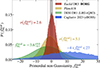 |
Fig. 1. Inference power of BORG on |


The paper is structured as follows. In Sect. 2, we provide an overview of the method and the algorithmic design choices. Emphasis has been placed on the galaxy bias model employed, the scale-dependent bias model, and on how the adiabatic curvature fluctuation maps were generated. In Sect. 3, we provide descriptions of the data generation setup and the datasets generated. Specifications for Euclid mock data and objectives of the Euclid mission with respect to PNG are included here. We finalise the section with the list of tests included in this project. We present the results in Sect. 4, which cover convergence results, results on fNL, and test-specific results. Finally, we summarise in Sect. 5, and discuss future work in Sect. 6.
2. Method
The primary goal of this paper is to forecast how well field-level inference can jointly constrain fNL and cosmic initial conditions in spectroscopic Euclid mock data. In this context, field-level inference uses the entirety of the 3D cosmic matter field and its formation history to optimally extract the available information from the data to constrain cosmology, such as primordial fluctuations or cosmological parameters (Jasche & Wandelt 2013; Leclercq & Heavens 2021; Baumann & Green 2022; Nguyen et al. 2021, 2024; Beyond-2pt Collaboration 2025). This is achieved by constructing a data model that forward models an arbitrary set of initial conditions, so that the corresponding predicted galaxy field can be directly compared with the data at the field level (Jasche et al. 2010; Jasche & Wandelt 2013; Seljak et al. 2017; Schmidt et al. 2019; Kostić et al. 2022; Porqueres et al. 2022; Andrews et al. 2023; Porqueres et al. 2023; Bayer et al. 2023; Stopyra et al. 2024). To test the performance of field-level inference, we set up a series of mock datasets, all emulating the survey features of the Euclid mission, including selection effects, window function, and galaxy number counts. Then, we analysed the mock datasets by running Markov chain Monte Carlo (MCMC) analyses in a Bayesian hierarchical framework. The MCMC runs produced plausible values of the primordial matter fluctuations, fNL, and marginalised nuisance parameters, all conditioned on the observed data. These outputs constitute the main results to make the said forecasts on fNL and the cosmic initial conditions.
In this section, we provide a more detailed description of the field-level inference algorithm used (Sect. 2.1). Next, we describe the applied PNG model (Sect. 2.2), and the galaxy bias model used (Sect. 2.3). In the following, we provide a brief description of how we ran the MCMC analyses. Finally, we outline the generation of inferred 3D maps of adiabatic curvature fluctuations (Sect. 2.5), which is a new data product presented for the first time, to our knowledge, in this paper.
2.1. Overview of BORG
The Bayesian Origin Reconstruction from Galaxies (BORG) algorithm is a Bayesian hierarchical inference framework and is designed for the analysis of cosmic structure in cosmological surveys through forward modelling of three-dimensional galaxy fields (Jasche & Wandelt 2013; Jasche et al. 2015; Lavaux & Jasche 2016; Jasche & Lavaux 2019; Lavaux et al. 2019). The forward model in BORG aims to recreate the physical process in which the galaxies formed and observed, as closely as possible to the underlying physical process. In other words, the data model connects the three-dimensional primordial matter field to the observed distribution of galaxies, effectively reformulating the inverse problem of inferring the initial conditions into a statistical forward problem. In practice, we still have to simplify the model that provides the local galaxy abundances through statistical mapping between the matter field and the galaxy distribution. Thus, the objective of BORG is, given the assumed forward model, to explore the joint posterior distribution of initial conditions (denoted as ϵ), cosmological parameters, and nuisance parameters, as constrained by the observed data. The problem can be formulated in the form of a joint posterior distribution 𝒫post(ϵ,fNL,{big}|NgO):
 (1)
(1)
where NgO are the observed data in the form of galaxy counts, {big} are the bias parameters, and 𝒫f, 𝒫ϵ, 𝒫b are the prior distributions. The prior in the white-noise field 𝒫ϵ(ϵ) is a Gaussian with zero mean and unit standard variance. The likelihood distribution 𝒫like(NgO|ϵ,fNL,{big}) is defined by the data model.
The data model forward evolves a set of initial conditions to the corresponding predicted galaxy field, in the form of galaxy number counts. The forward model starts by simulating the gravitational progression of the matter field over time through a structure formation model. This process yields a predicted realisation of the late-time dark matter field, which is populated using a galaxy bias model (Sect. 2.3, Andrews et al. 2023). The window function and survey selection effects are taken into account by evaluating the survey footprint and radial selection functions at each voxel. We note that while the sky map in this work consists of a binary selection function in the form of the survey footprint, BORG is able to account for more complex selection functions, such as those in the form of relative probabilities in each sky pixel (Lavaux et al. 2019). The resulting predicted galaxy field is compared to the observed galaxy field through a likelihood distribution. A schematic overview of the data model used in the BORG algorithm in this paper is given in Fig. 2. One feature to be specifically pointed out in the data model is that the primordial perturbation with fNL enters the data model at a different step from the evaluation of the structure formation model. This allows the algorithm to break the degeneracy between gravitational nonlinearities and primordial signals (Baumann & Green 2022; Andrews et al. 2023). To emphasise, a major advantage of relying on forward model analysis to infer PNG is that more information is available, beyond what is available for standard methods (Leclercq & Heavens 2021; Nguyen et al. 2024).
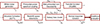 |
Fig. 2. Flow chart illustrating the forward model implemented in BORG (Jasche & Wandelt 2013; Andrews et al. 2023). The forward model connects a set of initial conditions to a model prediction. This output can then be compared to the data at the field level through a likelihood evaluation. The parameter under each box represents the output of the box and what is provided to the next step of the forward model. The parameters above some boxes represent the additional input of each computation. We especially highlight the inclusion of the |

To sample the joint posterior spanned by the data model, the algorithm relies on MCMC analysis. The complete multivariate distribution (Eq. (1)) is handled using a Gibbs sampling approach. The sampling scheme consists of a mixture of Hamiltonian Monte Carlo (HMC, Duane et al. 1987; Betancourt 2017) and slice sampling techniques (Hastings 1970; Neal 2003, 2011). To reiterate, the joint posterior distribution includes the three-dimensional initial density fields, cosmological parameters (i.e. fNL), and the galaxy bias parameters for each galaxy catalogue (see Sect. 3.2). Exploring this joint posterior distribution allows BORG to effectively leverage all available information in the data for optimal parameter constraints, while also marginalising over nuisance parameters, given the data model and its resolution. Thus, through an iterative MCMC analysis, BORG performs a statistically rigorous analysis, allowing us to quantify the significance of inferred quantities (Jasche & Wandelt 2013). The sampling scheme is given in Fig. 3.
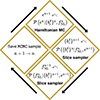 |
Fig. 3. Flow chart depicting the sampling scheme in BORG. The sampling scheme can be divided into four major parts: Sampling the 3D initial conditions, sampling the galaxy bias parameters (one set for each tracer catalogue), sampling the fNL parameter, and finally saving the data products and restarting the cycle. Each sub-box depicts the conditional posterior from which the sample is drawn, and the sampling technique that is used. |
For more details on the forward model and likelihood, we refer to the previous publication (Andrews et al. 2023). For a description of the structure formation model, second-order Lagrangian perturbation theory (2LPT), we refer to similar work (Jasche & Wandelt 2013; Jasche et al. 2015; Lavaux & Jasche 2016; Lavaux et al. 2019; Tsaprazi et al. 2022).
2.2. Model of local primordial non-Gaussianity fNL
Before applying the primordial perturbation with fNL, we first convolved the Gaussian white noise field ϵ with the primordial transfer function TG(k). The field ϵ is the set of initial conditions for the forward model shown in Fig. 2. The transfer function TG(k) scaled the white noise field so that it has the properties of the primordial power spectrum. In this work, we first generated the adiabatic curvature perturbation ℛ, with covariance set by the amplitude As, and, following the discrete primordial power spectrum, the resulting Gaussian potential field ϕG then has the following covariance:
 (2)
(2)
with V = L3 the volume of the data cube, a and b mesh indices, and  the Kronecker delta. The amplitude As set the variance of the primordial curvature perturbation ℛ, which we then converted to the Bardeen potential during matter domination via
  . This Gaussian potential field ϕg, evaluated at a → 0, provided the physical initial conditions for the forward model and contained full 3D information on the primordial matter fluctuations. The primordial gravitational potential in real space is then calculated with an inverse Fourier transform, with which we computed the perturbed primordial gravitational potential ΦNG. Generally, PNG is the deviation of the primordial gravitational potential from Gaussian statistics. To the lowest order, these deviations are parameterised by the quantity fNL. Although the deviation can have different shapes (Karagiannis et al. 2018), in this paper we focus on forecasting the constraining power of the local form (or squeezed shape). We parameterised fNL through the matter-era Bardeen potential (Hodges et al. 1990; Kofman 1991; Salopek & Bond 1990; Gangui et al. 1994; Verde et al. 2000; Wang & Kamionkowski 2000; Komatsu & Spergel 2001):
 (3)
(3)
where ϕg is a field described by Gaussian statistics, evaluated at the Lagrangian position. We considered fNL to be a constant parameter, independent of scale and any other parameter, including time. It is also the lowest order of PNG. We leave the incorporation of the higher-order expansion of PNG for future implementations (Jeong & Komatsu 2009; Roth & Porciani 2012; Leistedt et al. 2014).
2.3. Galaxy bias model
In galaxy survey analysis, galaxy formation is typically described as a functional relationship of the dark matter field and bias parameters (Assassi et al. 2015; Desjacques et al. 2018a). Specifically, we treated galaxies as ‘biased’ tracers of the dark matter field, meaning that they shared similar clustering statistics and properties. However, the true relationship is unknown and constitutes one of the most important unresolved problems in LSS cosmology (for an exhaustive review, see Desjacques et al. 2018a). Thus, while noting that the forecasts are highly dependent on the estimated relationship, we assumed a next-to-leading order bias model with scale-dependent bias components (Assassi et al. 2015; Barreira 2020). The motivation is that since we are still at relatively large scales (> 60 h−1 Mpc), a relationship between the dark matter field and the galaxy field can be described as a linear function. By further including additional terms beyond the linear bias, we allowed the model to account for nonlinear features as well.
The complete bias model for a given tracer population g adopted in this paper is defined as
![Mathematical equation: $$ \begin{aligned} \rho _{\rm g}(z, \boldsymbol{q}) = \left\langle N_{\rm g}^\mathrm{O} \, \right\rangle \, \Bigg [ 1 + b_1 \, \delta _{\rm m}(z)+ \frac{b_2}{2} \delta _{\rm m}^2(z) + b_{K} \, K^2(z) \nonumber \\ \quad \quad + \, b_\phi \, {f_\mathrm{NL} } \, \phi _{\rm g}(\boldsymbol{q}) + {b_{\phi ,\,\delta }} \, {f_\mathrm{NL} } \, \delta _{\rm m}(z) \, \phi _{\rm g} (\boldsymbol{q}) \Bigg ], \end{aligned} $$](/articles/aa/full_html/2026/07/aa53802-25/aa53802-25-eq19.gif) (4)
(4)
where  is the mean number of observed galaxies, b1 is the linear bias, b2 is the second-order bias, bK is the tidal field bias, and K2(z) =
 ![Mathematical equation: $ \rm{tr} \left [ K^2_{ij} (z) \right ] $](/articles/aa/full_html/2026/07/aa53802-25/aa53802-25-eq21.gif) , where
, where  is the long-wavelength tidal field (Lazeyras et al. 2021; Barreira et al. 2021)4. Scale-dependent bias terms bϕ and bϕ, δ are defined and further discussed in Sect. 2.3. We note that ϕ(q) is evaluated in Lagrangian space, while δm(z) is evaluated in a space that includes redshift-space distortions, which we call redshift space. In this project, we analyse the data at constant redshifts and thus do not account for effects that arise due to observing the galaxies on their light cones. We leave the inclusion of light-cone effects when inferring PNG to a future publication.
We assumed a fixed noise level for the Gaussian distribution of galaxies, set to  (Andrews et al. 2023). In an upcoming publication, we will assess both the noise-level assumption and the likelihood model for describing the distribution of galaxies at the voxel level. Additionally, we will explore how the constraints on fNL depend on these choices. The ground truth values of the galaxy parameters (used to generate the mock data) can be found in Table 1.
Detailed specifications of the spectroscopic Euclid mock data used in this paper.
We mention that there is also the possibility of using Effective Field Theory (EFT) to model the galaxy bias formalism and likelihood in a field-level inference approach (Schmidt et al. 2019, 2020; Schmidt 2021; Babić et al. 2022; Tucci & Schmidt 2024; Stadler et al. 2023; Babić et al. 2025; Nguyen et al. 2024; Stadler et al. 2025a,b; Kostić et al. 2023). For a review of the galaxy bias problem, the interested reader is referred to the literature (Desjacques et al. 2018a).
2.3.1. Scale-dependent bias model
In the model of local PNG considered, the primordial perturbation gives rise to a scale-dependent imprint on the biased tracer populations. This is due to the coupling of short- and long-wavelength modes in a non-zero fNL universe (Dalal et al. 2008; Slosar et al. 2008; Matarrese & Verde 2008; Carbone et al. 2008; Verde & Matarrese 2009). Thus, the PNG adds a scale-dependent contribution to the galaxy bias relation between galaxies and the underlying primordial gravitational field, which scales as ∝k−2 (Dalal et al. 2008; Slosar et al. 2008; Matarrese & Verde 2008; Carbone et al. 2008; Verde & Matarrese 2009), which is the most prominent on the largest scales. In this paper, we adopted the universal mass function (Barreira 2022c; Lucie-Smith et al. 2023; Fondi et al. 2024; Gutiérrez Adame et al. 2024) for a non-zero fNL universe. This allowed us to model the bias parameter of the primordial gravitational potential bϕ as a function of the linear bias b1
 (5)
(5)
with δc = 1.686 being the spherical critical overdensity in an Einstein–de Sitter universe (Percival 2005), and p a tracer-dependent parameter. For this forecast, we fixed p to 0.55 or 1 for each tracer population (Barreira et al. 2020; Cabass et al. 2022). Additionally, we incorporated the bias for the cross-field term bϕ, δ, adopting the parameterisation of Barreira (2022b) and Cabass et al. (2022)5,
![Mathematical equation: $$ \begin{aligned} {b_{\phi ,\,\delta }} = b_{\phi } - b_1 + 1 + \delta _{\rm c} \, \left[b_2 - \frac{8}{21} \, \left(b_1 - 1\right) \right]. \end{aligned} $$](/articles/aa/full_html/2026/07/aa53802-25/aa53802-25-eq25.gif) (6)
(6)
The problem of accurately modelling bϕ and bϕ, δ remains an unresolved challenge within the cosmological community (Biagetti 2019; Barreira 2022a; Achúcarro et al. 2022; Barreira & Krause 2023; Sullivan et al. 2023; Gutiérrez Adame et al. 2024; Fondi et al. 2024; Ding et al. 2024; Sullivan & Chen 2025; Kvasiuk et al. 2025). Improving the precision of the models for these bias parameters is crucial for robust and unbiased inference of fNL (Moradinezhad Dizgah et al. 2021; Barreira 2022c; Lazeyras et al. 2023). Further model-driven investigations of the treatment of bϕ and bϕ, δ will result in more robust and comprehensive models that better capture the underlying physical processes. In this paper, we adopt the universal mass approximation as a practical choice (Barreira 2020, 2022c). However, we emphasise that this assumption is not fundamental to the method itself, but as advances are achieved in the modelling of bϕ and bϕ, δ, the forward model will be revised accordingly. For a more in-depth discussion of the problem, see Moradinezhad Dizgah et al. (2021) and Barreira (2022c).
2.4. Running the MCMC analysis
The BORG algorithm performs a large-scale MCMC to explore the joint posterior distribution of Eq. (1), given the mock datasets. We briefly touch on the details of the MCMC analysis performed in this paper. We follow the prescription as in Ramanah et al. (2019) and Andrews et al. (2023), which provide more details.
To ensure that the sampler can sample from the target posterior distribution, we initialised the initial conditions ϵ at a randomly chosen point, set at one-tenth of the overall amplitude. The bias parameters are initialised at nine-tenths of their ground truth values, and fNL is shifted by +5. The prior distribution on fNL is a Gaussian distribution with μfNL = 0, σ(fNL) = 100. This design is motivated by the choice to have a broad and non-informative prior.
We started the burn-in phase of the MCMC runs by exclusively sampling the initial conditions ϵ, with fNL and the bias parameters kept constant to their starting values. This first step continued until the amplitude of the initial conditions fluctuated around the prior expectation. This was monitored by the power spectra estimated from Markov samples. For an example of such a plot, see the results of similar work (e.g. Porqueres et al. 2019a; Ramanah et al. 2019; Porqueres et al. 2022; Andrews et al. 2023). Next, we continued the run with sampling bias parameters, where each catalogue was assigned its own set, which were allowed to converge and stabilise. Finally, we included the sampling of fNL. To ensure the inclusion of only post-burn-in samples, additional 5000 samples were generated before including MCMC samples in the analysis. At this point, BORG explored the parameter space of plausible large-scale structure realisations, spanned by ϵ, fNL, and the bias parameters.
The MCMC chains were run until convergence, as determined by the Gelman–Rubin statistic  (Gelman & Rubin 1992). The Gelman–Rubin statistic is calculated by dividing the sequential samples of the chains into M distinct sets, each with an equal number of samples, where M typically ranges from 4 to 8. The sets were separated by N discarded samples, where N denotes the number of samples required to decorrelate fNL, to ensure statistical independence. More details on the autocorrelation length of fNL for each run can be found in Appendix B. When the threshold
  was reached, the chain was considered to have converged.
It should be noted that a proper Gelman–Rubin test assumes independent MCMC chains. In our case, a single MCMC chain has been split into several chains for the evaluation of the Gelman–Rubin test, due to limitations in computational resources. By doing this, we acknowledge the risks associated with this, for example, the sampler getting stuck in a local minimum or biasing our results. However, from investigating the convergence in the other diagnostic results (e.g. correlation lengths, corner plots, and estimates on uncertainty of uncertainty), we deem these risks to be negligible.
2.5. Generating 3D maps of adiabatic curvature fluctuations
Our field-level inference method, in addition to providing measurements of fNL, inferred the primordial gravitational potential. Given a posterior sample of ΦNG, we can generate a 3D map of the adiabatic curvature perturbation, or ℛ map (Planck Collaboration XVII 2016a). From Eqs. (2) and (3), we computed ΦNG(q) and then related it to the corresponding curvature field via the matter-era relation6.
 (7)
(7)
where q is the vector in Lagrangian space (Komatsu & Spergel 2001; Okamoto & Hu 2002; Lyth & Wands 2002; Sasaki et al. 2006). Since BORG sampled the posterior of ΦNG(q), we also estimated the corresponding uncertainties across the chain. The resulting ℛ maps are presented in Sect. 4.2, together with a detailed description of the dataset. For a 2D reconstruction of the adiabatic curvature field, see Sect. 6.3 in Planck Collaboration XVII (2016a).
3. Data and data generation
3.1. The Euclid Wide Survey and local primordial non-Gaussianity
The Euclid Wide Survey has among its goals to probe the expansion history and evolution of our Universe (Scaramella et al. 2014; Euclid Collaboration: Scaramella et al. 2022). To perform this task, Euclid will observe a region of 15 000 square degrees, over a redshift range of 0.9 < z < 1.8. Over the next six years, it will observe up to 30 million spectroscopic redshift galaxies with high precision (σz ≈ 0.001), which can be used for galaxy clustering studies.
Among several cosmological measurements, inferring PNG is one of the primary objectives of the Euclid mission. More specifically, we focus solely on the local shape of PNG (Eq. (3)). The earliest goals were set at σ(fNL)≈2 (68.3% CI). This forecast is based on statistical information from two-point correlation functions measured by spectroscopic redshift galaxies and for a ground truth value of  (Laureijs et al. 2011). However, more recent Fisher forecasts estimate that σ(fNL) around 4 to 5 (68.3% CI) is achievable, given the accuracy of the spectroscopic redshift measurements and updated galaxy counts (Amendola et al. 2018). These results include marginalisation over the galaxy bias parameters, nuisance parameters, and other cosmological parameters (Giannantonio et al. 2012; Amendola et al. 2018). We acknowledge that the constraining power of the forecasts is highly dependent on the measured linear galaxy bias b1 and the relationship bϕ(b1), due to the scale-dependent bias effect (as discussed in Sect. 2.3). That being said, the constraints on fNL × bϕ will be largely insensitive to this uncertainty (Barreira 2022a). Unless unspecified, we use the value of p = 0.55 (Euclid Collaboration: Finelli et al. 2026).
3.2. Euclid specifications
We base the mock datasets on the forecast specifications of Euclid, meaning that we made use of the survey features of the Euclid mission to generate the mock data. Examples include sky completeness coverage, radial selection effects, bias parameter values, and galaxy counts.
In Fig. 4, we illustrate the sky completeness map used. We emphasise that the same completeness map is used for all four galaxy catalogues, and has a total sky coverage of roughly 15 000 square degrees. Also, while the sky completeness map used in this forecast is the survey geometry footprint of the Euclid survey (Euclid Collaboration: Scaramella et al. 2022), BORG has the ability to use more complex sky completeness masks in its data model (Jasche & Lavaux 2019; Lavaux et al. 2019; Andrews et al. 2023).
 |
Fig. 4. Euclid sky map. This sky map illustrates the observed (yellow) and masked (red) regions for the Euclid survey of this project. The survey mask is a result of the observation strategy of the Euclid mission (Euclid Collaboration: Scaramella et al. 2022). We point out that each tracer catalogue uses one single survey strategy but extends outwards at different redshifts (as illustrated in Fig. 5). |
The radial selection functions are plotted in Fig. 5. The observed number counts are split into four different galaxy populations, each population corresponding to a catalogue. This design choice is based on the redshift binning of the Euclid forecasts (Euclid Collaboration: Blanchard et al. 2020). Here, it can be seen that each subsequent catalogue reaches further into the observable universe, covering a nonoverlapping redshift range 0.9 < z < 1.8. The number counts decrease towards higher redshifts.
 |
Fig. 5. Euclid radial selection function. This plot displays the normalised radial selection, dN(z)/(dΩ dz), for the four galaxy catalogues in this project. Notice how the tracer catalogues do not overlap but rather cover separate regions in the mock universe. |
The values of the galaxy bias parameters and number densities are listed in Table 1. These bias values were chosen as in Table 1 of Yankelevich & Porciani (2019), which constitutes the current estimate of the bias values as a function of redshift. The number densities were based on Table 3 of Euclid Collaboration: Blanchard et al. (2020). The values for the scale-dependent bias parameters were derived with Eqs. (5) and (6).
3.3. Mock data generation
To generate mock data, we follow similar procedures as described in previous works (Jasche & Kitaura 2010; Jasche & Wandelt 2013; Ramanah et al. 2019; Andrews et al. 2023). In general, these mock datasets were generated by running the forward model on a set of randomly drawn initial conditions. Thus, the same forward model is used for both mock data generation and the inference process, maintaining no model mismatch. We provide the details below, in a step-by-step description.
-
The evaluation of the physics forward model was prepared for a cubic Cartesian box of side length L = 8000 h−1 Mpc and Ngrid = 32, 64, 128, or 256, yielding grid resolutions in the range of ΔL = 250 h−1 Mpc, ΔL = 125 h−1 Mpc, ΔL = 62.5 h−1 Mpc, and ΔL = 31.25 h−1 Mpc, respectively.
-
A random three-dimensional field ϵ, with zero mean and unit standard deviation, was generated. Given this white-noise field, a primordial density field was computed by applying the primordial power spectrum (Eq. (2)), perturbing it with the fNL parameter (Eq. (3)), and then apply the cosmological transfer function as provided by CLASS (Lesgourgues & Tram 2014). This produced the linear matter field δL, which was the starting point for the gravitational structure formation model.
-
To reduce the sample variance of the particle distribution, we oversampled the initial density by a factor of 2 per dimension, resulting in a total number of (2N)3 simulation particles. Particles were evolved to the present epoch using 2LPT. Redshift-space distortions were then applied by performing an additional displacement of the particles along the line of sight, proportional to their 2LPT peculiar velocities, thereby mapping the particle distribution from real space to redshift space. The particles were subsequently assigned to a three-dimensional Cartesian grid via the Cloud-In-Cell (CIC) kernel to obtain the present-day three-dimensional matter density field δm in redshift space.
-
To emulate a biased galaxy distribution, we applied a next-to-leading order, scale-dependent galaxy bias (as described in Sect. 2.3) to the forward-modelled density field. The output is the galaxy field, wherein the galaxy counts in each voxel are characterised by a Gaussian distribution. Detailed specifications are organised in Table 1, including the parameter choices for the galaxy bias model.
-
Finally, the radial selection functions and the survey geometry were applied to the simulated galaxy field to emulate the observational effects of the survey.
We used the set of best-fit cosmological parameters (Ωm = 0.3153, ΩΛ = 0.6847, Ωb = 0.0493, h = 0.6736, As = 2.1 × 10⁻⁹, ns = 0.9649) from Planck (Planck Collaboration VI 2020c) to calculate the cosmological power spectrum and transfer functions. A summary of the specifications, including detailed parameter choices for the galaxy bias model, is provided in Table 1. We provide a rendering of one of the mock datasets in Appendix C. We note that by relying on 2LPT to model structure formation we forego including small-scale physics that capture information at higher-order correlation functions beyond the bispectrum. To accurately and completely capture these higher-order effects at small-scales, in future publications, we will rely on N-body solvers, such as tCOLA (Tassev et al. 2013), particle mesh (Jasche & Lavaux 2019), or field-level emulators (Doeser et al. 2024). Since the data analysis in this paper is self-consistent with the mock data generation – using the same forward model for both inference and mock data creation – it captures all the information contained in the mock datasets.
Finally, we note that our inference formally includes modes close to the Nyquist frequency of the initial conditions grid. These scales are not fully converged, since their true nonlinear evolution would in reality be influenced by unresolved fluctuations at smaller scales. While this does not introduce a bias in our analysis, as the treatment is self-consistent, the unconverged modes remain well below the noise level and are therefore not expected to affect the inference. However, their inclusion may still lead to an optimistic estimate of the constraining power on fNL. A more conservative treatment would involve downweighting these modes through, for example, a scale-dependent noise prescription, which we leave for future work.
3.4. Overview of runs
In this section, we provide a complete list of the runs that we performed for this paper. Although the main aim of this paper is to forecast fNL measurements with mock Euclid galaxy surveys, we are also interested in investigating the performance of the method in various configurations. To achieve this, we vary the specifications in the data and the analysis (e.g. resolution, marginalisation, and parameters values). The main questions for each test, together with the design of the runs, are outlined in the following list. For a concise overview of the runs in this project, we refer to Table 2.
-
Resolution study
The imprint of PNG affects the full cosmic matter field, both at large and small scales. To test the method’s constraining power as a function of scale, we set up three different runs. The first at coarser grid resolution (ΔL = 250 h−1 Mpc, Run #1), one at medium grid resolution (ΔL = 125 h−1 Mpc, Run #2), one at finer grid resolution (ΔL = 62.5 h−1 Mpc, Run #3), and one at higher grid resolution (ΔL = 31.25 h−1 Mpc, Run #4). By increasing the voxel resolution, we allow the algorithm to have more degrees of freedom in describing the 3D cosmic matter field. Therefore, we expect that the method can use more small-scale information in the LSS to constrain fNL. We also perform these runs as a benchmark as we adjust other parameters, for example, changing the sampling scheme or parameter values.
-
fNL = 0, fNL = 5
We aim to investigate whether the algorithm’s constraining power depends on the fiducial amplitude of PNG. To test this, we generated two identical mock datasets that differ only by their values of fNL: one with fNL = 0 (Run #3) and the other with fNL = 5 (Run #5), both with finer grid resolutions. In this way, we test the algorithm roughly in the upper 68.3% CI of the Planck 2018 measurement and the other in null detection (Planck Collaboration IX 2020b). This also allows us to check if the algorithm can accurately retrieve a non-zero ground truth value of
 .
. -
p = 1
We aim to investigate how much the algorithm’s constraining power depends on the amplitude of the scale-dependent bias effect. To test this, we generate and analyse mock data that have p (Eq. (5)) set to 1 (Run #6) instead of 0.55 (which is the default for the other runs). Since this value of p is larger, there is a weaker scale-dependent bias amplitude in this analysis, meaning that the expectation is that the inferred uncertainty in fNL will be larger.
-
Sampling bϕ, bϕ, δ
As described in Sect. 2.3, PNG gives rise to a scale-dependent bias effect that is modelled by bϕ and bϕ, δ. In the other runs, we fix bϕ and bϕ, δ to the expressions of the universal mass function (Eqs. (5) and (6)). In this test, we want to test whether the algorithm is able to jointly sample fNL, bϕ and bϕ, δ, in the presence of priors. Therefore, in Run #7, we include the sampling of bϕ and bϕ, δ, in addition to the initial conditions ϵ, fNL, and the other bias parameters. In the mock data, the ground truth values of bϕ and bϕ, δ are set to the universal expressions of the mass function. The priors for bϕ and bϕ, δ are Gaussians centred on universal mass function expressions (as a function of b1 and b2), with standard deviations set to 40% of their values:
 , and
, and  , where
  and
and  are the expressions in Eqs. (5) and (6). We note that b1 and b2 used to evaluate
  and
and  correspond to the values in the current state of the MCMC chain, rather than the ground truth values of
  and
and  . We are mainly interested in evaluating the performance of the method, in terms of σ(fNL), and investigating possible correlations between bias parameters bϕ and bϕ, δ, and fNL. If successful, this run further highlights the flexibility of the field-level inference approach in adjusting the galaxy bias model, and to sample bias parameters arising due to primordial effects.
Overview of the runs included in this project.
4. Results
The main goal of this work is to infer the marginal posterior distribution of fNL for each generated mock dataset. In this way, we provide both forecasts of how well BORG can constrain fNL with the Euclid Wide Survey, and test the inference power under a variety of configurations. The results have been summarised in Table 3. For each run, we obtain an ensemble of samples, each containing plausible values of fNL, the initial conditions, and the nuisance parameters, given the mock data. From these ensembles, we calculate the ensemble mean and uncertainty of fNL and include these in the table. We also compute the uncertainty of the uncertainty, which quantifies the margin of error. For completeness, we also include the ground truth  values, the resolution, and the corresponding kmax, which we define as the Nyquist frequency, kNF7. We highlight that each inferred ensemble mean ⟨fNL⟩ is within the 68.3% CI of the ground truth
  value.
Inferred fNL for each run.
The main run of this project, Run #4, constitutes the most realistic Euclid mock data. With it, we infer fNL at a voxel resolution of 31.25 h−1 Mpc  . We illustrate the inferred posterior distribution in Fig. 6, with which we find fNL = 0.3 ± 2.6. This marginal posterior distribution contains the entirety of the information available in the data, given the physics model and resolution.
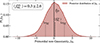 |
Fig. 6. Field-level results for inferring fNL for a high-resolution run (Run #4). The figure illustrates that the method can find a unimodal marginalised distribution of fNL that best explains the data, with the ground truth value |

Furthermore, for a visual comparison between the runs, we include Fig. 7, with all the inferred marginal posterior distributions of fNL. To maintain legibility, we have divided the seven posteriors into two subplots.
 |
Fig. 7. Field-level results for inferring fNL for all runs. The first four runs, Runs #1–#4, are included in panel a. The last three runs, Runs #5–#7, are included in panel b. The marginal distribution of Run #5 has been shifted to be relative to the ground truth |

4.1. Further tests
Below, we present the results for the tests outlined in Sect. 3.4. In Sect. 4.2, we describe and present the results of generating maps of adiabatic curvature fluctuations.
4.1.1. Resolution study
We discuss the results of the resolution investigation, in which we test the constraining power of BORG as a function of the available small scales. This is tested by comparing Runs #1–4. As can be seen, by increasing the resolution from 323 to 643, we improve the results by roughly 42%. Furthermore, by increasing the resolution from 643 to 1283, we improve the results by roughly 32%. Finally, by increasing the resolution from 1283 to 2563, we improve the constraining power by approximately 40%. We note that we are still at the mildly linear regime ( ), but we use a forward model that can account for nonlinearities in the data. This means that we can, in principle, further increase the resolution while still being able to model the emerging nonlinear small-scale physics. However, due to the computational cost, we leave this investigation to a future project.
4.1.2. fNL = 0 and fNL = 5
We outline the results for the performance of the algorithm for a non-zero ground truth value of  . We generate two different mock datasets with the same white noise and galaxy bias parameters but with different fNL values. These two are Run #3
  and Run #5
  . The results show that the constraints for the two runs are similar, which indicates that the algorithm’s performance is largely independent of the underlying fNL value. Moreover, the uncertainty of the uncertainty std[σ(fNL)] is similar for the two runs, providing additional confirmation of this. The results indicate that our algorithm does not have a strong bias or performance issue related to ground truth
  , which means that we expect the same sensitivity for a null signal or a primordial signal. We leave the exploration of sensitivity to large ground truth values of
  to a future project, which previous work has shown can influence the estimated uncertainty (Creminelli et al. 2007; Liguori et al. 2007).
4.1.3. Amplitude of scale-dependent bias effect
We discuss the results of weakening the effect of the scale-dependent bias in the model, by changing the parameter p. We perform two runs at the same resolution, but with differing values of p from 0.55 (Run #2) to 1 (Run #6). The results show that by increasing p we reduce the constraining power in fNL. In fact, the change in p from 0.55 to 1 results in a decrease in the constraints of roughly 39%. This outcome highlights the dependence of the algorithm forecast on changes in scale-dependent bias parameters.
4.1.4. Sampling of bϕ and bϕ, δ
With this investigation, we want to test the flexibility of BORG to include the joint sampling of the scale-dependent bias parameters, including priors. This is relevant since it is still not fully understood how to model the scale-dependent bias effect (Barreira & Krause 2023). We present the results of Run #7, in which we include the sampling of bϕ and bϕ, δ, in addition to the initial conditions, fNL, and the other parameters of the galaxy bias. The results show that BORG is still able to provide unbiased constraints on fNL, but that the constraints degrade by approximately 20%. In Fig. 8, we provide a visualisation of the corner plot of the sampled fNL and galaxy bias parameters of the fourth catalogue in the Markov chain. The corner plots for the other catalogues and the full correlation matrix are presented and discussed in Appendix B. Although the results show promise, further developments and choice of priors (for example the ones presented in Fondi et al. 2024; Gutiérrez Adame et al. 2024) will be investigated in a future publication.
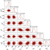 |
Fig. 8. Field-level results for inferring fNL, when simultaneously also sampling bϕ and bϕ, δ. Corner plot for fNL and bias parameters, for Run #7, catalogue 4. Although the priors (described in Sect. 3.4) keep the inferred value of fNL centering around the expected value of 0, the possible degeneracies with bϕ and bϕ, δ are still explored. Thus, while the results indicate that our field-level inference method can jointly sample fNL together with bϕ and bϕ, δ (in the presence of priors), more work is needed to stabilise the region of explored fNL values. The priors on bϕ and bϕ, δ is centred around their Gaussians centred on universal mass function expressions, with standard deviations at 40% of that value: |


4.2. Maps of adiabatic fluctuations
In addition to measuring fNL, our field-level inference method infers the initial 3D conditions of the data. With these sets of plausible initial conditions, we generate maps of the 3D adiabatic curvature fluctuations of the post-inflationary universe. To generate maps of adiabatic curvature fluctuations, we apply Eq. (7) to a subset of the inferred samples of Run #4. The subset consists of every tenth sample from the Markov chain, starting from the first sample after the burn-in phase has concluded. By analysing the posterior ensemble, we can compute the average ℛ field and the corresponding variance. We mention that we also include the inferred values of fNL in the evaluation of the perturbed primordial gravitational potential ΦNG. These estimated statistical 3D fields constitute a novel data product that the method enables.
In Fig. 9, we render the 2D projections (in the x direction) of the resulting 3D maps. We also include the ground truth ℛ field of the mock data and the absolute residual between the inferred and ground truth field. The upper-left panel illustrates the ground truth map of ℛ provided by the mock data. The upper-right panel illustrates the average inferred ℛ values. The bottom-left panel illustrates the uncertainty in the inferred adiabatic curvature fluctuations, whereas the bottom-right panel depicts the residual between the ground truth and the inferred. To highlight the effect of the selection function, the edges of the survey are marked with dotted lines, with voxels outside the edge completely masked in Eulerian space. The voxels inside the edges are regions of the data that are unmasked or only partially masked. However, we emphasise that BORG is capable of extrapolating information into unobserved voxels using the physics-informed data model (Jasche & Wandelt 2013; Leclercq et al. 2015; Jasche et al. 2015; Leclercq et al. 2017). In summary, these maps offer a comprehensive representation of plausible adiabatic curvature fluctuations and capture the statistical properties and (at least the three-point) correlation functions of these fluctuations.
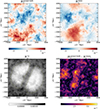 |
Fig. 9. Illustrations of the inferred adiabatic curvature fluctuations. For each saved sample, we have a set of initial conditions ϵ that produce a plausible set of model predictions, constrained by the data. Each set of initial conditions corresponds to a field of adiabatic curvature fluctuations (Eqs. (2) and (7)), which are the input to the structure formation model. By computing these fluctuations for a subset of the chain, the method can provide an expected estimate of the fluctuation of the adiabatic curvature along with uncertainty. We highlight the edge of the survey window with the dotted lines, meaning that voxels outside of the inner regions in the final observed field contain no observations. In the top-left plot, we have included the ground truth field of adiabatic curvature fluctuations used to generate the mock data, averaged over the x direction. In the top-right plot, we have the expectation value of the adiabatic curvature fluctuations averaged over the x direction. In the bottom-left plot, we have the corresponding uncertainty averaged over the x direction. Lastly, in the bottom-right plot, we include the absolute difference between the mean inferred field and the ground truth field. |
4.2.1. Additional diagnostics of the runs
Before concluding, we briefly mention the additional diagnostics and results of the runs provided in the appendix. In Appendix B we present correlation matrices, correlation lengths, and corner plots of fNL and the bias parameters for Run #4 and #7. In Appendix C, we highlight the generated mock data and illustrate the inferred final density fields and compare them with their ground truth representations. We present further tests of the adiabatic curvature fluctuations, including plots, in Appendix A.
5. Discussion
The detection of PNG would have profound implications for our understanding of the early Universe and the inflationary paradigm. Local PNG can serve as a powerful probe to test the single-field inflation hypothesis (Falk et al. 1993; Gangui et al. 1994; Komatsu & Spergel 2001; Maldacena 2003; Bartolo et al. 2004; Chen 2010; Biagetti 2019; Meerburg et al. 2019; Green et al. 2024). In this context, the local fNL parameter provides a convenient parameterisation to quantify the lowest order of PNG. Projects such as Euclid aim at constraining fNL with high-precision redshift surveys (Laureijs et al. 2011; Amendola et al. 2018; Euclid Collaboration: Finelli et al. 2026). To forecast the detectable level of PNG in Euclid data, we apply a field-level inference method on Euclid-like spectroscopic mock data to constrain fNL. This approach allows us to naturally and jointly use all of the information available in the data to provide measurements of PNG and the primordial matter fluctuations.
To generate and infer fNL from the mock data, we use BORG, which is a Bayesian hierarchical field-level inference algorithm designed to analyse galaxy redshift surveys. The data model for this project, illustrated in Fig. 2, forward models the primordial matter fluctuations to a predicted observation of the 3D galaxy field, so that the initial conditions can be directly inferred from the data. The data model captures all the effects of the perturbation of the primordial gravitational potential with fNL and the scale-dependent bias effect on the final observable. We point out that we still assume the universal mass approximation (Moradinezhad Dizgah & Keating 2019; Barreira 2022b) and lowest-order fNL contributions. The data model will be updated as more progress is made in modelling the scale-dependent bias effect. Our approach can handle a variety of observational and systematic effects in the forward model, providing robust inferences of PNG and the early Universe (Jasche & Lavaux 2017; Porqueres et al. 2019b; Lavaux et al. 2019). Moreover, the explicit physics-informed data model allows the method to maintain interpretability (Jasche & Wandelt 2013; Porqueres et al. 2019b) and perform posterior predictive tests of the results (Jasche & Lavaux 2019; Lavaux et al. 2019).
In this study, we use Euclid forecast specifications to generate mock data, such as the number of galaxies, number of catalogues, observed volume, and redshift binning, among others. To generate the mock data, we employed a forward model on a white-noise field, including effects such as structure formation effects, redshift selection functions, and sky masks, allowing us to simulate realistic observations. Throughout the study, we generate and analyse mock data under a variety of conditions, for example, tests with different ground truth  values, and with different resolutions. The investigations paint a comprehensive picture of the impact of various factors on the inference process.
This study demonstrates the successful sampling of the parameter fNL using mock Euclid data. All the runs carried out for this analysis result in inferred values of fNL within the 68.3% CI of the ground truth  value. These constraints demonstrate the reliability and robustness of the inference methodology. In particular, at a resolution of 31.25 h−1 Mpc, we achieve a constraining power of σ(fNL) = 2.6 (68.3% CI). The resolution study carried out in this paper demonstrates the ability of our method to use information on small scales to constrain fNL. In addition, we present detailed maps of primordial adiabatic curvatures, or ℛ maps, and their corresponding uncertainties, providing a comprehensive rendering of the inferred initial conditions. In general, these results highlight the potential of using field-level inference to constrain primordial physics with Euclid data.
We forecast how well BORG can constrain fNL in mock Euclid spectroscopic datasets. We highlight our major findings below and thereafter provide a summary.
-
The field-level inference framework successfully handles Euclid-like specifications, accommodating the large survey volume, the number of galaxies, and various physical effects and noise properties. The data model used includes the generation of primordial gravitational potential, perturbation with local PNG, running a structure formation computation, applying a bias model, and evaluating the likelihood of galaxy formation.
-
Our primary finding is that, at a resolution of 31.25 h−1 Mpc(kNF = 0.1 h Mpc−1), our method achieves an uncertainty of σ(fNL) = 2.6 for fNL = 0 at 68.3% CI, assuming the universal mass function and p = 0.55.
-
Our method can infer the parameter fNL with high precision at multiple resolutions, different fiducial fNL values, and sampling configurations, demonstrating the consistency and versatility of the methodology.
-
As we increase the resolution, our algorithm provides tighter constraints on fNL, confirming the results in Andrews et al. (2023, see Figure 7). Thus, we expect additional improvements by further increasing the resolution, especially since our data model is capable of handling nonlinearities beyond the considered kNF.
-
When the amplitude of the scale-dependent bias effect is weakened, from p = 0.55 to p = 1, the constraints on the inferred fNL decrease by approximately 40% (68.3% CI).
-
We perform a run by also sampling the scale-dependent bias parameters bϕ and bϕ, δ, with priors centred on Eqs. (5) and (6). The run provides unbiased constraints on fNL, but with an increase in σ(fNL) by approximately 20% (68.3% CI).
-
At a resolution of 31.25 h−1 Mpc, we generate maps of adiabatic curvature fluctuations from inferred initial conditions, offering valuable data products for conducting further investigations into the early Universe.
-
We showcase additional convergence tests and data products, for example corner plots, correlation lengths, and inferred cosmic fields, in Appendices B–C.
In conclusion, our method provides a complementary and independent approach to statistical summary estimators for constraining primordial physics in galaxy redshift surveys. By using the full formation history of the Universe in the data model, field-level inference opens up the possibility to perform optimal measurements of PNG up to the given resolution and data model. With these measurements, the scientific community will be able to significantly reduce the parameter space of plausible models for the inflationary universe. In this way, our method will contribute to the scientific success of the Euclid mission by enabling it to excel in one of its primary research objectives.
6. Future work
In this section, we provide a discussion on the further testing and development of the method for inferring primordial physics in galaxy redshift survey data, with a focus on the following aspects: (1) validation against the Euclid flagship simulation (Potter et al. 2017; Euclid Collaboration: Castander et al. 2025), (2) handling observational effects such as relativistic effects and foreground systematic effects, and (3) inclusion of additional inflationary model parameters and (4) cosmological parameters.
6.1. Method validation with the Euclid flagship simulation
Before analysing the upcoming observed data, further tests of the adopted data model against more complex data are required, for example against the Euclid flagship simulation. The Euclid flagship simulation is a gravity-only dark matter simulation consisting of 12 6003 dark matter particles within the size of 3780 h−1 Mpc. With the method, one can use the simulated halo catalogue as a substitute for galaxies, and thus perform further tests on the data model and the performance of the algorithm in constraining fNL. Examples include further testing of the structure formation model and bias model in BORG, and how well they can capture the results of the full simulation. Furthermore, analysing N-body simulations with non-zero fNL values is another way to validate the implemented PNG model (Jung et al. 2022; Coulton et al. 2023; Jung et al. 2023a,b; Fondi et al. 2024; Hadzhiyska et al. 2024). In addition, another insightful investigation is to test how changes in the data model, such as the choice of structure formation model, impact the algorithm’s inference power on fNL. Successfully further testing the algorithm with N-body simulations is a crucial step before the subsequent application on the upcoming real data.
6.2. Handling more complex observational effects
Real observational data are subject to various survey systematic and observational effects. Future work will therefore have to incorporate and mitigate these effects in the analysis framework. One example is the consideration of general relativistic effects, which imprint an effect similar to PNG on large scales. Another is the modelling of light-cone effects, which account for the evolution of the observable universe over cosmic time (Bruni et al. 2012; Jeong et al. 2012; Schmidt et al. 2013; Bertacca et al. 2014a,b; Jeong & Schmidt 2015; Yoo 2014; Yoo & Gong 2016; Koyama et al. 2018; Desjacques et al. 2018b; Umeh et al. 2019; Lavaux et al. 2019; Wang et al. 2020; Maartens et al. 2021; Martinez-Carrillo et al. 2021; Castorina & Di Dio 2022; Enríquez et al. 2022; Shiveshwarkar et al. 2023; Rossiter et al. 2025; Addis et al. 2025). By properly handling these effects, the algorithm aims to break the degeneracy between these effects and PNG, in such a way that one can ensure that the method accurately captures the relevant information from observed data. Furthermore, foreground systematic effects, such as contamination from Galactic emissions or instrumental artefacts, can significantly bias the measured cosmological parameters if they are not taken into account (Leistedt et al. 2014; Rezaie et al. 2021; Mueller et al. 2021; Rezaie et al. 2024). Developing robust methods to identify and marginalise these systematic effects is a key question in the Euclid mission. In addition, a careful treatment of velocity bias is required when modelling tracer dynamics in redshift space. While negligible on the largest scales relevant for PNG, velocity bias and related higher-order RSD effects become important at intermediate scales (kmax > 0.05 h Mpc−1), particularly if one aims to perform the inference at higher resolutions, such as the resolutions of run #4. Extending or adjusting the bias model to properly capture these effects will be crucial to ensure unbiased cosmological constraints (Stadler et al. 2023, 2025a,b). Lastly, tests incorporating photometric redshift datasets will also be conducted (Jasche & Wandelt 2012; Tsaprazi et al. 2023).
6.3. Inclusion of additional inflationary model parameters
Inflationary models offer a rich framework for understanding the early Universe and its subsequent evolution. To further constrain the space of plausible inflationary models, the data model can be extended to include additional inflationary model parameters beyond the parameter fNL. For example, the data model could include other parameters such as the local trispectrum non-Gaussianity parameter gNL (Okamoto & Hu 2002; Sasaki et al. 2006; Jeong & Komatsu 2009; Leistedt et al. 2014; Roth & Porciani 2012; Shiveshwarkar et al. 2024; Pardede et al. 2023), the running-of-the-scalar index αs (Fedeli et al. 2010; Planck Collaboration X 2020a; Germán 2021), and other shapes of PNG, for example, the equilateral non-Gaussianity parameter  (Babich et al. 2004; Scoccimarro et al. 2012; Regan et al. 2012; Planck Collaboration XXIV 2014a; Schmidt et al. 2015; Planck Collaboration XVII 2016a; Karagiannis et al. 2018; Planck Collaboration IX 2020b; Karagiannis et al. 2020; Baumann & Green 2022). Such implementations would be subject to validation tests and mock data studies before making predictions on how well field-level inference methods can constrain such parameters in the large-scale structure. In short, by incorporating additional primordial parameters, the data model would be able to perform a more thorough exploration of the inflationary paradigm in the data, and thus allowing the method to further distinguish different inflationary models.
6.4. Joint sampling of cosmological parameters
Another test of interest is to explore the parameter space of the ΛCDM model together with non-Gaussian cosmic initial conditions. By doing so, one would be ale to assess the efficacy of field-level inference in the context of jointly sampling other cosmological parameters together with fNL. Examples of such parameters include Ωm, w0 (Ramanah et al. 2019), and σ8 (Schmidt 2021; Porqueres et al. 2021, 2022, 2023; Nguyen et al. 2024; Beyond-2pt Collaboration 2025). However, extending the analysis to include additional degrees of freedom exposes the algorithm to potential parameter degeneracies, which could degrade the constraints in fNL. Based on previous work, we anticipate a marginal decline in performance, projected to be within the limit of 10% (Jung et al. 2023a,b). Confirmation of these expectations will be made through future mock data tests, within the context of Euclid simulations and other datasets.
Acknowledgments
We thank Fabian Schmidt for valuable feedback on the manuscript. JJ acknowledges support by the Swedish Research Council (VR) under the project 2020-05143 – ‘Deciphering the Dynamics of Cosmic Structure’ and from the contract ASI/ INAF for the Euclid mission n.2018-23-HH.0. GL acknowledge financial support from the Centre National d’Etudes Spatiales (project GCEUCLID), and the Simons Foundation collaboration programme ‘Learning the Universe’. FF, MB, and DP acknowledge partial financial support from the contract ASI/ INAF for the Euclid mission n.2018-23-HH.0 and from the INFN InDark initiative. The computations and data handling were enabled by resources provided by the National Academic Infrastructure for Supercomputing in Sweden (NAISS) and the Swedish National Infrastructure for Computing (SNIC) at Tetralith partially funded by the Swedish Research Council through grant agreements no. 2022-06725 and no. 2018-05973. This research utilised the HPC facility supported by the Technical Division of the Department of Physics, Stockholm University. MB acknowledges financial support from the INFN InDark initiative and from the COSMOS network through the ASI (Italian Space Agency) Grants 2016-24-H.0 and 2016-24-H.1-2018, as well as 2020-9-HH.0 (participation in LiteBIRD phase A). JV was supported by Ruth och Nils–Erik Stenbäcks Stiftelse and Research Council of Finland grant 347088. FP acknowledges partial support from the INFN grant InDark and the Departments of Excellence grant L.232/2016 of the Italian Ministry of University and Research (MUR) and the FCT project with ref. number PTDC/FIS-AST/0054/2021. We acknowledge the use of the following packages: NumPy (Harris et al. 2020), Matplotlib (Hunter 2007), GetDist (Lewis 2019), and HEALPix (Gorski et al. 2005). This work is done within the Aquila Consortium (https://www.aquila-consortium.org/). The Euclid Consortium acknowledges the European Space Agency and a number of agencies and institutes that have supported the development of Euclid, in particular the Agenzia Spaziale Italiana, the Austrian Forschungsförderungsgesellschaft funded through BMIMI, the Belgian Science Policy, the Canadian Euclid Consortium, the Deutsches Zentrum für Luft- und Raumfahrt, the DTU Space and the Niels Bohr Institute in Denmark, the French Centre National d’Etudes Spatiales, the Fundação para a Ciência e a Tecnologia, the Hungarian Academy of Sciences, the Ministerio de Ciencia, Innovación y Universidades, the National Aeronautics and Space Administration, the National Astronomical Observatory of Japan, the Netherlandse Onderzoekschool Voor Astronomie, the Norwegian Space Agency, the Research Council of Finland, the Romanian Space Agency, the Swiss Space Office (SSO) at the State Secretariat for Education, Research, and Innovation (SERI), and the United Kingdom Space Agency. A complete and detailed list is available on the Euclid web site (https://www.euclid-ec.org/consortium/community/).
References
- Abazajian, K. N., Adshead, P., Ahmed, Z., et al. 2016, arXiv e-prints [arXiv:1610.02743] [Google Scholar]
- Achúcarro, A., Biagetti, M., Braglia, M., et al. 2022, arXiv e-prints [arXiv:2203.08128] [Google Scholar]
- Acquaviva, V., Bartolo, N., Matarrese, S., et al. 2003, Nucl. Phys. B, 667, 119 [NASA ADS] [CrossRef] [Google Scholar]
- Addis, C., Guandalin, C., & Clarkson, C. 2025, JCAP, 04, 080 [Google Scholar]
- Alvarez, M., Baldauf, T., Bond, J. R., et al. 2014, arXiv e-prints [arXiv:1412.4671] [Google Scholar]
- Amendola, L., Appleby, S., Avgoustidis, A., et al. 2018, Liv. Rev. Relat., 21, 2 [Google Scholar]
- Andrews, A., Jasche, J., Lavaux, G., et al. 2023, MNRAS, 520, 5746 [Google Scholar]
- Arkani-Hamed, N., & Maldacena, J. 2015, arXiv e-prints [arXiv:1503.08043] [Google Scholar]
- Assassi, V., Baumann, D., & Schmidt, F. 2015, JCAP, 12, 043 [Google Scholar]
- Babić, I., Schmidt, F., & Tucci, B. 2022, JCAP, 08, 007 [Google Scholar]
- Babić, I., Schmidt, F., & Tucci, B. 2025, JCAP, 11, 066 [Google Scholar]
- Babich, D., Creminelli, P., & Zaldarriaga, M. 2004, JCAP, 08, 009 [Google Scholar]
- Baldauf, T., Seljak, U., & Senatore, L. 2011a, JCAP, 04, 006 [Google Scholar]
- Baldauf, T., Seljak, U., Senatore, L., et al. 2011b, JCAP, 10, 031 [Google Scholar]
- Ballardini, M., Matthewson, W. L., & Maartens, R. 2019, MNRAS, 489, 1950 [NASA ADS] [CrossRef] [Google Scholar]
- Barberi Squarotti, M., Camera, S., & Maartens, R. 2024, JCAP, 02, 043 [Google Scholar]
- Barreira, A. 2020, JCAP, 12, 031 [Google Scholar]
- Barreira, A. 2022a, JCAP, 11, 013 [Google Scholar]
- Barreira, A. 2022b, JCAP, 01, 033 [Google Scholar]
- Barreira, A. 2022c, JCAP, 04, 057 [Google Scholar]
- Barreira, A., & Krause, E. 2023, JCAP, 10, 044 [Google Scholar]
- Barreira, A., Cabass, G., Schmidt, F., et al. 2020, JCAP, 12, 013 [NASA ADS] [CrossRef] [Google Scholar]
- Barreira, A., Lazeyras, T., & Schmidt, F. 2021, JCAP, 08, 029 [CrossRef] [Google Scholar]
- Bartolo, N., Komatsu, E., Matarrese, S., et al. 2004, Phys. Rep., 402, 103 [NASA ADS] [CrossRef] [Google Scholar]
- Baumann, D., & Green, D. 2022, JCAP, 08, 061 [Google Scholar]
- Baumann, D., Jackson, M. G., Adshead, P., et al. 2009, AIP Conf. Proc., 1141, 10 [NASA ADS] [CrossRef] [Google Scholar]
- Bayer, A. E., Seljak, U., & Modi, C. 2023, arXiv e-prints [arXiv:2307.09504] [Google Scholar]
- Bermejo-Climent, J. R., Demina, R., Krolewski, A., et al. 2025, A&A, 698, A177 [NASA ADS] [CrossRef] [EDP Sciences] [Google Scholar]
- Bertacca, D., Maartens, R., & Clarkson, C. 2014a, JCAP, 09, 037 [Google Scholar]
- Bertacca, D., Maartens, R., & Clarkson, C. 2014b, JCAP, 11, 013 [Google Scholar]
- Betancourt, M. 2017, arXiv e-prints [arXiv:1701.02434] [Google Scholar]
- Beyond-2pt Collaboration (Krause, E., et al.) 2025, ApJ, 990, 99 [Google Scholar]
- Biagetti, M. 2019, Galaxies, 7, 71 [Google Scholar]
- Biagetti, M., Calles, J., Castiblanco, L., et al. 2022, JCAP, 10, 002 [CrossRef] [Google Scholar]
- Brown, Z., Demina, R., Adame, A. G., et al. 2025, MNRAS, 543, 2078 [Google Scholar]
- Bruni, M., Crittenden, R., Koyama, K., et al. 2012, Phys. Rev. D, 85, 041301 [NASA ADS] [CrossRef] [Google Scholar]
- Byrnes, C. T., & Choi, K.-Y. 2010, Adv. Astron., 2010, 724525 [Google Scholar]
- Byrnes, C. T., Choi, K.-Y., & Hall, L. M. H. 2009, JCAP, 02, 017 [Google Scholar]
- Byrnes, C. T., Gerstenlauer, M., Nurmi, S., et al. 2010, JCAP, 10, 004 [Google Scholar]
- Cabass, G., Ivanov, M. M., Philcox, O. H. E., et al. 2022, Phys. Rev. Lett., 129, 021301 [Google Scholar]
- Cagliari, M. S., Castorina, E., Bonici, M., et al. 2024, JCAP, 08, 036 [Google Scholar]
- Carbone, C., Verde, L., & Matarrese, S. 2008, ApJ, 684, L1 [Google Scholar]
- Castorina, E., & Di Dio, E. 2022, JCAP, 01, 061 [CrossRef] [Google Scholar]
- Castorina, E., Hand, N., Seljak, U., et al. 2019, JCAP, 09, 010 [Google Scholar]
- Celoria, M., & Matarrese, S. 2018, arXiv e-prints [arXiv:1812.08197] [Google Scholar]
- Chaussidon, E., de Mattia, A., Yèche, C., et al. 2025a, JCAP, 01, 135 [Google Scholar]
- Chaussidon, E., Yèche, C., de Mattia, A., et al. 2025b, JCAP, 06, 029 [Google Scholar]
- Chen, X. 2010, Adv. Astron., 2010, 638979 [NASA ADS] [CrossRef] [Google Scholar]
- Chen, X., Ebadi, R., & Kumar, S. 2022, JCAP, 08, 083 [Google Scholar]
- Chen, X., Padmanabhan, N., & Eisenstein, D. J. 2025, JCAP, 08, 055 [Google Scholar]
- Coulton, W. R., Villaescusa-Navarro, F., Jamieson, D., et al. 2023, ApJ, 943, 64 [NASA ADS] [CrossRef] [Google Scholar]
- Creminelli, P., & Zaldarriaga, M. 2004, JCAP, 10, 006 [Google Scholar]
- Creminelli, P., Senatore, L., & Zaldarriaga, M. 2007, JCAP, 03, 019 [Google Scholar]
- Creminelli, P., D’Amico, G., Musso, M., et al. 2011, JCAP, 11, 038 [Google Scholar]
- Dalal, N., Doré, O., Huterer, D., et al. 2008, Phys. Rev. D, 77, 123514 [CrossRef] [Google Scholar]
- D’Amico, G., Lewandowski, M., Senatore, L., et al. 2025, Phys. Rev. D, 111, 063514 [Google Scholar]
- Desjacques, V., Jeong, D., & Schmidt, F. 2018a, Phys. Rep., 733, 1 [Google Scholar]
- Desjacques, V., Jeong, D., & Schmidt, F. 2018b, JCAP, 12, 035 [Google Scholar]
- Ding, S., Lavaux, G., & Jasche, J. 2024, A&A, 690, A236 [NASA ADS] [CrossRef] [EDP Sciences] [Google Scholar]
- Doeser, L., Jamieson, D., Stopyra, S., et al. 2024, MNRAS, 535, 1258 [NASA ADS] [CrossRef] [Google Scholar]
- Doré, O., Bock, J., Ashby, M., et al. 2014, arXiv e-prints [arXiv:1412.4872] [Google Scholar]
- Duane, S., Kennedy, A. D., Pendleton, B. J., et al. 1987, Phys. Lett. B, 195, 216 [CrossRef] [Google Scholar]
- Duivenvoorden, A. J., Meerburg, P. D., & Freese, K. 2020, Phys. Rev. D, 102, 023521 [Google Scholar]
- Enríquez, M., Hidalgo, J. C., & Valenzuela, O. 2022, JCAP, 03, 048 [Google Scholar]
- Euclid Collaboration (Ballardini, M., et al.) 2024, A&A, 683, A220 [NASA ADS] [CrossRef] [EDP Sciences] [Google Scholar]
- Euclid Collaboration (Blanchard, A., et al.) 2020, A&A, 642, A191 [NASA ADS] [CrossRef] [EDP Sciences] [Google Scholar]
- Euclid Collaboration (Castander, F. J., et al.) 2025, A&A, 697, A5 [Google Scholar]
- Euclid Collaboration (Finelli, F., et al.) 2026, A&A, in press, https://doi.org/10.1051/0004-6361/202556600 [Google Scholar]
- Euclid Collaboration (Ilić, S., et al.) 2022, A&A, 657, A91 [CrossRef] [EDP Sciences] [Google Scholar]
- Euclid Collaboration (Mellier, Y., et al.) 2025, A&A, 697, A1 [Google Scholar]
- Euclid Collaboration (Scaramella, R., et al.) 2022, A&A, 662, A112 [NASA ADS] [CrossRef] [EDP Sciences] [Google Scholar]
- Falk, T., Rangarajan, R., & Srednicki, M. 1993, ApJ, 403, L1 [Google Scholar]
- Fedeli, C., Finelli, F., & Moscardini, L. 2010, MNRAS, 407, 1842 [Google Scholar]
- Finelli, F., Bucher, M., Achúcarro, A., et al. 2018, JCAP, 04, 016 [Google Scholar]
- Fishman, G., & Yarberry, S. 1997, INFORMS J. Comput., 9, 3 [Google Scholar]
- Fondi, E., Verde, L., Villaescusa-Navarro, F., et al. 2024, JCAP, 02, 048 [Google Scholar]
- Friedrich, O., Uhlemann, C., Villaescusa-Navarro, F., et al. 2020, MNRAS, 498, 464 [NASA ADS] [CrossRef] [Google Scholar]
- Gangui, A., Lucchin, F., Matarrese, S., et al. 1994, ApJ, 430, 447 [Google Scholar]
- Gelman, A., & Rubin, D. B. 1992, Stat. Sci., 7, 457 [Google Scholar]
- Germán, G. 2021, Int. J. Mod. Phys. D, 30, 2150038 [Google Scholar]
- Giannantonio, T., & Percival, W. J. 2014, MNRAS, 441, L16 [NASA ADS] [CrossRef] [Google Scholar]
- Giannantonio, T., Porciani, C., Carron, J., et al. 2012, MNRAS, 422, 2854 [Google Scholar]
- Giri, U., Münchmeyer, M., & Smith, K. M. 2025, Phys. Rev. D, 112, 123544 [Google Scholar]
- Goldstein, S., Esposito, A., Philcox, O. H. E., et al. 2022, Phys. Rev. D, 106, 123525 [Google Scholar]
- Goldstein, S., Philcox, O. H. E., Hill, J. C., et al. 2024, Phys. Rev. D, 109, 043515 [Google Scholar]
- Gorski, K. M., Hivon, E., Banday, A. J., et al. 2005, ApJ, 622, 759 [Google Scholar]
- Graham, M. L., Connolly, A. J., Ivezić, Ž., et al. 2018, AJ, 155, 1 [Google Scholar]
- Green, D., Guo, Y., Han, J., et al. 2024, JCAP, 05, 090 [Google Scholar]
- Guth, A. H. 1981, Phys. Rev. D, 23, 347 [Google Scholar]
- Gutiérrez Adame, A., Avila, S., Gonzalez-Perez, V., et al. 2024, A&A, 689, A69 [NASA ADS] [CrossRef] [EDP Sciences] [Google Scholar]
- Hadzhiyska, B., Garrison, L. H., Eisenstein, D. J., et al. 2024, Phys. Rev. D, 109, 103530 [NASA ADS] [CrossRef] [Google Scholar]
- Harris, C. R., Millman, K. J., van der Walt, S. J., et al. 2020, Nature, 585, 357 [NASA ADS] [CrossRef] [Google Scholar]
- Hastings, W. K. 1970, Biometrika, 57, 97 [Google Scholar]
- Ho, S., Agarwal, N., Myers, A. D., et al. 2015, JCAP, 05, 040 [Google Scholar]
- Hodges, H. M., Blumenthal, G. R., Kofman, L. A., et al. 1990, Nucl. Phys. B, 335, 197 [Google Scholar]
- Hunter, J. D. 2007, Comput. Sci. Eng., 9, 90 [NASA ADS] [CrossRef] [Google Scholar]
- Huterer, D., Cunha, C. E., & Fang, W. 2013, MNRAS, 432, 2945 [Google Scholar]
- Jasche, J., & Kitaura, F. S. 2010, MNRAS, 407, 29 [NASA ADS] [CrossRef] [Google Scholar]
- Jasche, J., & Lavaux, G. 2017, A&A, 606, A37 [NASA ADS] [CrossRef] [EDP Sciences] [Google Scholar]
- Jasche, J., & Lavaux, G. 2019, A&A, 625, A64 [NASA ADS] [CrossRef] [EDP Sciences] [Google Scholar]
- Jasche, J., & Wandelt, B. D. 2012, MNRAS, 425, 1042 [CrossRef] [Google Scholar]
- Jasche, J., & Wandelt, B. D. 2013, MNRAS, 432, 894 [Google Scholar]
- Jasche, J., Kitaura, F. S., Wandelt, B. D., et al. 2010, MNRAS, 406, 60 [NASA ADS] [CrossRef] [Google Scholar]
- Jasche, J., Leclercq, F., & Wandelt, B. D. 2015, JCAP, 01, 036 [Google Scholar]
- Jeong, D., & Komatsu, E. 2009, ApJ, 703, 1230 [NASA ADS] [CrossRef] [Google Scholar]
- Jeong, D., & Schmidt, F. 2015, Class. Quant. Grav., 32, 044001 [Google Scholar]
- Jeong, D., Schmidt, F., & Hirata, C. M. 2012, Phys. Rev. D, 85, 023504 [NASA ADS] [CrossRef] [Google Scholar]
- Jung, G., Karagiannis, D., Liguori, M., et al. 2022, ApJ, 940, 71 [Google Scholar]
- Jung, G., Karagiannis, D., Liguori, M., et al. 2023a, ApJ, 948, 135 [Google Scholar]
- Jung, G., Ravenni, A., Baldi, M., et al. 2023b, ApJ, 957, 50 [Google Scholar]
- Jung, G., Ravenni, A., Liguori, M., et al. 2024, ApJ, 976, 109 [Google Scholar]
- Kalaja, A., Meerburg, P. D., Pimentel, G. L., et al. 2021, JCAP, 04, 050 [Google Scholar]
- Karagiannis, D., Lazanu, A., Liguori, M., et al. 2018, MNRAS, 478, 1341 [NASA ADS] [CrossRef] [Google Scholar]
- Karagiannis, D., Slosar, A., & Liguori, M. 2020, JCAP, 11, 052 [Google Scholar]
- Karagiannis, D., Fonseca, J., Maartens, R., et al. 2021, Phys. Dark Universe, 32, 100821 [Google Scholar]
- Karagiannis, D., Maartens, R., Fonseca, J., et al. 2024, JCAP, 03, 034 [Google Scholar]
- Kofman, L. 1991, Phys. Scr. Vol. T, 36, 108 [Google Scholar]
- Komatsu, E. 2010, Class. Quant. Grav., 27, 124010 [CrossRef] [Google Scholar]
- Komatsu, E., & Spergel, D. N. 2001, Phys. Rev. D, 63, 063002 [NASA ADS] [CrossRef] [Google Scholar]
- Komatsu, E., Afshordi, N., Bartolo, N., et al. 2009, arXiv e-prints [arXiv:0902.4759] [Google Scholar]
- Kostić, A., Jasche, J., Ramanah, D. K., et al. 2022, A&A, 657, L17 [NASA ADS] [CrossRef] [EDP Sciences] [Google Scholar]
- Kostić, A., Nguyen, N.-M., Schmidt, F., et al. 2023, JCAP, 07, 063 [Google Scholar]
- Koyama, K., Umeh, O., Maartens, R., et al. 2018, JCAP, 07, 050 [Google Scholar]
- Krolewski, A., Percival, W. J., Ferraro, S., et al. 2024, JCAP, 03, 021 [Google Scholar]
- Kvasiuk, Y., Münchmeyer, M., & Smith, K. 2025, Phys. Rev. D, 112, 023540 [Google Scholar]
- Laureijs, R., Amiaux, J., Arduini, S., et al. 2011, arXiv e-prints [arXiv:1110.3193] [Google Scholar]
- Lavaux, G., & Jasche, J. 2016, MNRAS, 455, 3169 [Google Scholar]
- Lavaux, G., Jasche, J., & Leclercq, F. 2019, arXiv e-prints [arXiv:1909.06396] [Google Scholar]
- Lazeyras, T., Barreira, A., & Schmidt, F. 2021, JCAP, 10, 063 [CrossRef] [Google Scholar]
- Lazeyras, T., Barreira, A., Schmidt, F., et al. 2023, JCAP, 01, 023 [Google Scholar]
- Leclercq, F., & Heavens, A. 2021, MNRAS, 506, L85 [Google Scholar]
- Leclercq, F., Jasche, J., Lavaux, G., & Wandelt, B. 2015, arXiv e-prints [arXiv:1512.02242] [Google Scholar]
- Leclercq, F., Jasche, J., Lavaux, G., et al. 2017, JCAP, 06, 049 [Google Scholar]
- Leistedt, B., Peiris, H. V., & Roth, N. 2014, Phys. Rev. Lett., 113, 221301 [NASA ADS] [CrossRef] [Google Scholar]
- Lesgourgues, J., & Tram, T. 2014, JCAP, 09, 032 [Google Scholar]
- Lewis, A. 2019, arXiv e-prints [arXiv:1910.13970] [Google Scholar]
- Liguori, M., Yadav, A., Hansen, F. K., et al. 2007, Phys. Rev. D, 76, 105016 [Google Scholar]
- LoVerde, M., Miller, A., Shandera, S., et al. 2008, JCAP, 04, 014 [Google Scholar]
- LSST Science Collaborations (Abell, P. A., et al.) 2009, arXiv e-prints [arXiv:0912.0201] [Google Scholar]
- Lucie-Smith, L., Barreira, A., & Schmidt, F. 2023, MNRAS, 524, 1746 [NASA ADS] [CrossRef] [Google Scholar]
- Lyth, D. H., & Wands, D. 2002, Phys. Lett. B, 524, 5 [Google Scholar]
- Maartens, R., Jolicoeur, S., Umeh, O., et al. 2021, JCAP, 04, 013 [Google Scholar]
- Maldacena, J. 2003, J. High Energy Phys., 5, 013 [Google Scholar]
- Martinez-Carrillo, R., Hidalgo, J. C., Malik, K. A., et al. 2021, JCAP, 12, 025 [Google Scholar]
- Matarrese, S., & Verde, L. 2008, ApJ, 677, L77 [NASA ADS] [CrossRef] [Google Scholar]
- McCarthy, F., Madhavacheril, M. S., & Maniyar, A. S. 2023, Phys. Rev. D, 108, 083522 [Google Scholar]
- McQuinn, M. 2021, JCAP, 06, 024 [Google Scholar]
- Meerburg, P. D., Green, D., Flauger, R., et al. 2019, BAAS, 51, 107 [NASA ADS] [Google Scholar]
- Moradinezhad Dizgah, A., & Keating, G. K. 2019, ApJ, 872, 126 [Google Scholar]
- Moradinezhad Dizgah, A., Biagetti, M., Sefusatti, E., et al. 2021, JCAP, 05, 015 [CrossRef] [Google Scholar]
- Mueller, E.-M., Percival, W. J., & Ruggeri, R. 2019, MNRAS, 485, 4160 [Google Scholar]
- Mueller, E. M., Rezaie, M., Percival, W. J., et al. 2021, arXiv e-prints [arXiv:2106.13725] [Google Scholar]
- Münchmeyer, M., Madhavacheril, M. S., Ferraro, S., et al. 2019, Phys. Rev. D, 100, 083508 [Google Scholar]
- Neal, R. 2011, Handbook of Markov Chain Monte Carlo, 1st edn. (Chapman and Hall/CRC), 113 [Google Scholar]
- Neal, R. M. 2003, Ann. Stat., 31, 705 [Google Scholar]
- Nguyen, N.-M., Schmidt, F., Lavaux, G., et al. 2021, JCAP, 03, 058 [Google Scholar]
- Nguyen, N.-M., Schmidt, F., Tucci, B., et al. 2024, Phys. Rev. Lett., 133, 221006 [CrossRef] [Google Scholar]
- Okamoto, T., & Hu, W. 2002, Phys. Rev. D, 66, 063008 [Google Scholar]
- Pardede, K., Di Dio, E., & Castorina, E. 2023, JCAP, 09, 030 [Google Scholar]
- Percival, W. J. 2005, A&A, 443, 819 [NASA ADS] [CrossRef] [EDP Sciences] [Google Scholar]
- Peron, M., Jung, G., Liguori, M., et al. 2024, JCAP, 07, 021 [Google Scholar]
- Planck Collaboration XXIV. 2014a, A&A, 571, A24 [NASA ADS] [CrossRef] [EDP Sciences] [Google Scholar]
- Planck Collaboration XXII. 2014b, A&A, 571, A22 [NASA ADS] [CrossRef] [EDP Sciences] [Google Scholar]
- Planck Collaboration XVII. 2016a, A&A, 594, A17 [NASA ADS] [CrossRef] [EDP Sciences] [Google Scholar]
- Planck Collaboration XX. 2016b, A&A, 594, A20 [NASA ADS] [CrossRef] [EDP Sciences] [Google Scholar]
- Planck Collaboration X. 2020a, A&A, 641, A10 [NASA ADS] [CrossRef] [EDP Sciences] [Google Scholar]
- Planck Collaboration IX. 2020b, A&A, 641, A9 [Google Scholar]
- Planck Collaboration VI. 2020c, A&A, 641, A6 [NASA ADS] [CrossRef] [EDP Sciences] [Google Scholar]
- Porqueres, N., Jasche, J., Lavaux, G., et al. 2019a, A&A, 630, A151 [NASA ADS] [CrossRef] [EDP Sciences] [Google Scholar]
- Porqueres, N., Kodi Ramanah, D., Jasche, J., et al. 2019b, A&A, 624, A115 [NASA ADS] [CrossRef] [EDP Sciences] [Google Scholar]
- Porqueres, N., Heavens, A., Mortlock, D., et al. 2021, MNRAS, 502, 3035 [NASA ADS] [CrossRef] [Google Scholar]
- Porqueres, N., Heavens, A., Mortlock, D., et al. 2022, MNRAS, 509, 3194 [Google Scholar]
- Porqueres, N., Heavens, A., Mortlock, D., et al. 2023, arXiv e-prints [arXiv:2304.04785] [Google Scholar]
- Potter, D., Stadel, J., & Teyssier, R. 2017, Comput. Astrophys. Cosmol., 4, 2 [NASA ADS] [CrossRef] [Google Scholar]
- Ramanah, D. K., Lavaux, G., Jasche, J., et al. 2019, A&A, 621, A69 [NASA ADS] [CrossRef] [EDP Sciences] [Google Scholar]
- Regan, D. M., Schmittfull, M. M., Shellard, E. P. S., et al. 2012, Phys. Rev. D, 86, 123524 [Google Scholar]
- Rezaie, M., Ross, A. J., Seo, H.-J., et al. 2021, MNRAS, 506, 3439 [Google Scholar]
- Rezaie, M., Ross, A. J., Seo, H.-J., et al. 2024, MNRAS, 532, 1902 [NASA ADS] [CrossRef] [Google Scholar]
- Riquelme, W., Avila, S., García-Bellido, J., et al. 2023, MNRAS, 523, 603 [NASA ADS] [CrossRef] [Google Scholar]
- Rossiter, S. J., Camera, S., Clarkson, C., et al. 2025, JCAP, 07, 055 [Google Scholar]
- Roth, N., & Porciani, C. 2012, MNRAS, 425, L81 [Google Scholar]
- Salopek, D. S., & Bond, J. R. 1990, Phys. Rev. D, 42, 3936 [NASA ADS] [CrossRef] [Google Scholar]
- Sasaki, M., Väliviita, J., & Wands, D. 2006, Phys. Rev. D, 74, 103003 [Google Scholar]
- Scaramella, R., Mellier, Y., Amiaux, J., et al. 2014, Proc. Int. Astron. Union, 10, 375 [Google Scholar]
- Schmidt, F. 2021, JCAP, 04, 032 [Google Scholar]
- Schmidt, F., Jeong, D., & Desjacques, V. 2013, Phys. Rev. D, 88, 023515 [CrossRef] [Google Scholar]
- Schmidt, F., Chisari, N. E., & Dvorkin, C. 2015, JCAP, 10, 032 [Google Scholar]
- Schmidt, F., Elsner, F., Jasche, J., et al. 2019, JCAP, 01, 042 [Google Scholar]
- Schmidt, F., Cabass, G., Jasche, J., et al. 2020, JCAP, 11, 008 [Google Scholar]
- Schmittfull, M., & Seljak, U. 2018, Phys. Rev. D, 97, 123540 [NASA ADS] [CrossRef] [Google Scholar]
- Scoccimarro, R. 2000, ApJ, 542, 1 [Google Scholar]
- Scoccimarro, R., Sefusatti, E., & Zaldarriaga, M. 2004, Phys. Rev. D, 69, 103513 [Google Scholar]
- Scoccimarro, R., Hui, L., Manera, M., et al. 2012, Phys. Rev. D, 85, 083002 [NASA ADS] [CrossRef] [Google Scholar]
- Seljak, U. 2009, Phys. Rev. Lett., 102, 021302 [NASA ADS] [CrossRef] [Google Scholar]
- Seljak, U., Aslanyan, G., Feng, Y., et al. 2017, JCAP, 12, 009 [Google Scholar]
- Shiveshwarkar, C., Brinckmann, T., Loverde, M., et al. 2023, Phys. Rev. D, 108, 103538 [Google Scholar]
- Shiveshwarkar, C., Brinckmann, T., & Loverde, M. 2024, JCAP, 05, 094 [Google Scholar]
- Slosar, A., Hirata, C., Seljak, U., et al. 2008, JCAP, 08, 031 [Google Scholar]
- Stadler, J., Schmidt, F., & Reinecke, M. 2023, JCAP, 10, 069 [Google Scholar]
- Stadler, J., Schmidt, F., & Reinecke, M. 2025a, JCAP, 04, 089 [Google Scholar]
- Stadler, J., Schmidt, F., Reinecke, M., et al. 2025b, JCAP, 11, 055 [Google Scholar]
- Starobinsky, A. A. 1980, Phys. Lett. B, 91, 99 [Google Scholar]
- Stopyra, S., Peiris, H. V., Pontzen, A., et al. 2024, MNRAS, 527, 1244 [Google Scholar]
- Sullivan, J. M., & Chen, S.-F. 2025, JCAP, 03, 016 [Google Scholar]
- Sullivan, J. M., Prijon, T., & Seljak, U. 2023, JCAP, 08, 004 [Google Scholar]
- Tassev, S., Zaldarriaga, M., & Eisenstein, D. J. 2013, JCAP, 06, 036 [CrossRef] [Google Scholar]
- Tsaprazi, E., Nguyen, N.-M., Jasche, J., et al. 2022, JCAP, 08, 003 [CrossRef] [Google Scholar]
- Tsaprazi, E., Jasche, J., Lavaux, G., & Leclercq, F. 2023, arXiv e-prints [arXiv:2301.03581] [Google Scholar]
- Tucci, B., & Schmidt, F. 2024, JCAP, 05, 063 [Google Scholar]
- Uhlemann, C., Pajer, E., Pichon, C., et al. 2018, MNRAS, 474, 2853 [NASA ADS] [CrossRef] [Google Scholar]
- Umeh, O., Koyama, K., Maartens, R., et al. 2019, JCAP, 05, 020 [Google Scholar]
- Verde, L., & Matarrese, S. 2009, ApJ, 706, L91 [Google Scholar]
- Verde, L., Wang, L., Heavens, A. F., et al. 2000, MNRAS, 313, 141 [Google Scholar]
- Verde, L., Jimenez, R., Kamionkowski, M., et al. 2001, MNRAS, 325, 412 [Google Scholar]
- Wang, L., & Kamionkowski, M. 2000, Phys. Rev. D, 61, 063504 [Google Scholar]
- Wang, M. S., Beutler, F., & Bacon, D. 2020, MNRAS, 499, 2598 [Google Scholar]
- Yankelevich, V., & Porciani, C. 2019, MNRAS, 483, 2078 [NASA ADS] [CrossRef] [Google Scholar]
- Yip, J. H. T., Biagetti, M., Cole, A., et al. 2024, JCAP, 09, 034 [Google Scholar]
- Yoo, J. 2014, Phys. Rev. D, 90, 123507 [Google Scholar]
- Yoo, J., & Gong, J.-O. 2016, Phys. Lett. B, 754, 94 [Google Scholar]
Some improvements may arise from small-scale polarisation measurements (Baumann et al. 2009; Abazajian et al. 2016; Duivenvoorden et al. 2020; Kalaja et al. 2021), but these are not expected to reach the science target of σ(fNL) = 1 (Meerburg et al. 2019).
Examples include scale-dependent bias, higher-order statistics in the density field, mass distribution of tracers, and velocity field imprints.
See, for example, Porqueres et al. (2019b) and Lavaux et al. (2019).
Kij is computed in Fourier space, where the differential operators correspond to multiplications by components of the wavevector k.
We note that alternative parameterisations of bϕ, δ exist in the literature, for example Moradinezhad Dizgah et al. (2021) and D’Amico et al. (2025).
On super-Hubble scales, the general relation between the curvature perturbation and the Bardeen potential is ℛk = −[(5 + 3w)/(3 + 3w)] Φk, with w the equation-of-state parameter of the dominant component. During matter domination (w = 0) this reduces to the standard convention  , which we adopt throughout this work.
Here we take kmax to be the Nyquist frequency associated with the grid resolution. Modes near this scale are affected by discretisation and do not carry the full physical information, but this definition provides a convenient and consistent cut-off for comparison purposes.
Appendix A: Additional tests of the adiabatic curvature fluctuations
To further test our generated data products, we compute how well they relate to the ground truth adiabatic curvature field. We compare the power spectra of the ensemble-predicted adiabatic curvature fluctuations with the ground truth. The results can be seen in Fig. A.1. Furthermore, in each voxel, we have stored three values: i) the ground truth value (from the mock data itself), ii) the mean inferred estimate, and iii) the uncertainty of the estimate, which is given in terms of σ(ℛ). Thus, in the range of voxels, we evaluate whether the ground truth value is within the CIs 68.3%, 95.4%, or 99.7%. Our results show that in the 2563 voxels, 69.7 % are in the 1σ(ℛ) range, 95.6 % are in the 2σ(ℛ) range and 99.8 % are in the 3σ(ℛ) range. The test also shows that roughly 49 % of the inferred voxels fall above the ground truth value, while 51 % of the inferred voxels fall below the ground truth value. Thus, our inferred ℛ maps are representative of the ground truth ℛ map, to the expected confidence.
 |
Fig. A.1. Ensemble power spectra statistics of the inferred adiabatic curvature fluctuations, relative to the ground truth. The grey region is the 68% scatter around the mean power spectrum of the ensemble. |
Figs. A.2– A.5: We present the ensemble statistics of the adiabatic curvature fluctuation maps, in the Mollweide projection, for a distance of r = 2250 h−1 Mpc. The fields shown are the averages of the ground truth, the mean inferred, the standard deviation of the inferred, and the residuals between the ground truth and inferred in a single direction. The fields are multiplied by the selection value in each direction, effectively setting the masked directions to zero.
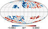 |
Fig. A.2. Mollweide projection of the ground truth adiabatic curvature fluctuation map. The projection is computed for a distance of r = 2250 h−1 Mpc, for an observer placed in the centre of the cube, and multiplied by the window selection function. |
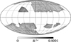 |
Fig. A.4. Similar to Fig A.2, but for the uncertainty of the inferred adiabatic curvature fluctuation map. |
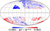 |
Fig. A.5. Similar to Fig A.2, but for the residual adiabatic curvature fluctuation map, defined as ℛground truth − ℛmean inferred. |
Appendix B: Tests of the algorithm
This section presents additional plots to offer further insight into the algorithm’s performance. The plots encompass autocorrelation lengths, correlation matrices, and corner plots that illustrate the relationships between fNL and the galaxy bias parameters.
Figure B.1 shows the autocorrelation lengths for fNL from all chains. The autocorrelation length is a metric used in MCMC algorithms to assess how quickly the samples in the chain become independent. Longer lengths indicate slower convergence, necessitating more iterations for reliable parameter estimates. On the contrary, shorter lengths denote faster convergence with reduced reliance on past samples. This metric is vital for evaluating MCMC efficiency, which impacts parameter estimation speed and computational requirements. In particular, the correlation length of fNL in the chains is approximately 10 000 samples for each chain, excluding Run #5.
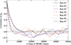 |
Fig. B.1. Correlation length of all chains, illustrating the rate at which samples in the various chains achieve independence. The typical correlation length for the chains is around 10 000 samples when bias parameters are also sampled. |
The correlation matrix summarises the relationships between variables in a dataset. It shows the magnitudes and direction of linear associations between pairs of variables. High positive values indicate strong positive correlations, while high negative values imply strong negative correlations. A correlation close to zero suggests a weak or no linear relationship. This matrix can also be used to identify potential degeneracies. The Pearson correlation coefficient rij is defined as:
 (B.1)
(B.1)
Here, Xi and Xj are the bias parameters or fNL, cov(Xi,Xj) is the covariance, and σi and σj are the standard deviations. As can be seen in Figs. B.2 and B.3, the galaxy bias parameters exhibit little or no correlations with fNL.
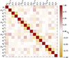 |
Fig. B.2. Correlation matrix of Run #4 (the primary run). The correlation matrix illustrates the pairwise relationships among variables, with colour-coding indicating the strength and direction of correlations, aiding in the identification of patterns and dependencies within the dataset. The results show little to no correlation, except for a mild anti-correlation between fNL and the linear bias values. |
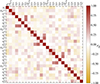 |
Fig. B.3. Correlation matrix of Run #7 (which includes the sampling of the scale-dependent bias parameters, bϕ and bϕ, δ). Colour coding indicates the strength and direction of the correlations, illustrating the little to no correlation between fNL and the non-linear bias parameters, including the scale-dependent bias parameters. |
On the same note, the corner plot depicts the interaction between the fNL and galaxy bias parameters and offers a visual representation of their joint distribution and correlations. This plot, visualised in Figs. B.4–B.7, B.8–B.10, and 8 displays the marginal distributions of each parameter on the diagonal and their joint distributions on the off-diagonal. It illustrates how changes in one parameter are associated with changes in the other, providing information on potential relationships and regions of interest between fNL and galaxy bias.
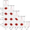 |
Fig. B.4. Corner plot for fNL and bias parameters, for Run #4, catalogue 1. The corner plot displays the joint distributions and marginal distributions of the variables in the multidimensional dataset covered by fNL and the bias parameters. Each subplot captures the relationships between pairs of variables, offering an overview of the dataset structure and dependencies. For the main run, there are few to no degeneracies in the bias parameters. |
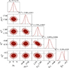 |
Fig. B.5. Corner plot for fNL and bias parameters, for Run #4, catalogue 2. Similar to Fig. B.4, there are little to no degeneracies between fNL and the bias parameters. |
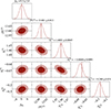 |
Fig. B.6. Corner plot for fNL and bias parameters, for Run #4, catalogue 3. Similar to Fig. B.4, there are little to no degeneracies between fNL and the bias parameters. |
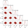 |
Fig. B.7. Corner plot for fNL and bias parameters, for Run #4, catalogue 4. Similar to Fig. B.4, there are few to no degeneracies between fNL and the bias parameters. |
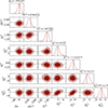 |
Fig. B.8. Corner plot for fNL and bias parameters, for Run #7, catalogue 1. Similar to Fig. B.4, there are little to no degeneracies between fNL and the bias parameters. |
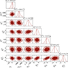 |
Fig. B.9. Corner plot for fNL and bias parameters, for Run #7, catalogue 2. Similar to Fig. B.4, there are little to no degeneracies between fNL and the bias parameters. |
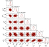 |
Fig. B.10. Corner plot for fNL and bias parameters, for Run #7, catalogue 3. Similar to Fig. B.4, there are few to no degeneracies between fNL and the bias parameters. |
Figure B.11 shows trace plots of the inferred values of fNL for the seven different runs, together with the corresponding effective sample sizes (ESS). Each panel displays the sampled values over the chains, along with the posterior mean and the 1σ interval. All chains fluctuate around a well-defined mean within the prior range, and no signs of long-term drifts or divergences are visible, indicating stable convergence. The ESS values, reported in the final panel, confirm that despite differences in chain length and correlation structure, the effective number of independent samples remains sufficiently large for reliable statistical inference. In particular, the main run, Run #4, shows good mixing properties. Overall, the combined diagnostics suggest that the inference of fNL is robust across different simulation setups, and that the recovered values are statistically stable.
 |
Fig. B.11. Trace plots of the inferred values of fNL for the seven runs. Each panel shows the thinned chains, displaying only every 1, 000th sample, with the raw chain in red, the posterior mean in black (solid line), and the 1σ interval in gray (dashed lines). The last panel summarises the effective sample sizes (ESS) for all runs, which are computed for the entire, unthinned chain. All chains exhibit stable convergence around well-defined mean values, with sufficiently large ESS to ensure reliable inference. |
Appendix C: Inferred density field and data projections
This section showcases plots of the inferred density fields and a comprehensive comparison by including the ground truth mock data fields.
Fig. C.1: We present the averages of the mock data field in three different directions. Notice how the data are cut due to the combination of the radial selection function and the completeness mask.
 |
Fig. C.1. Averaged projections of the mock data fields. The colour bar displays the number of galaxies in each pixel, which contains the sum of all galaxies in the summed-over axis. The image is intended to demonstrate the effects of the window function on the observed data and how the method can account for it. The galaxy field projected here is used for Run #4. Each pixel covers a width of 8000 h−1 Mpc/256 = 31.25 h−1 Mpc. |
Fig. C.2: We present the averages of the ground truth, the mean inferred, the variance of the inferred, and the residuals of the present-day dark matter field, δm, in a single direction.
 |
Fig. C.2. Averaged projections of the ground truth and statistical summaries of the inferred fields. The edge of the survey is highlighted with dotted lines, which means that voxels outside the edge are not observed. In the left panel, the ground truth density field is plotted. In the middle panel, the mean of the ensemble of the inferred fields is plotted. In the right panel, the standard deviation of the ensemble of the inferred fields is plotted. The image illustrates the method’s capability to recover the ground truth density field within the regions of observed data. We note that the voxels within the window selection function have less uncertainty and larger inferred means. The inferred fields are the product of Run #4. Each pixel covers a width and height of 8000 h−1 Mpc/256 = 31.25 h−1 Mpc. |
To emphasise, the core outcome of our method is the inferred fNL distribution; these inferred cosmic fields, with uncertainty estimates, stem from the byproduct of the field-level inference approach.
All Tables
Detailed specifications of the spectroscopic Euclid mock data used in this paper.
All Figures
|
Fig. 1. Inference power of BORG on |
| In the text | |
|
Fig. 2. Flow chart illustrating the forward model implemented in BORG (Jasche & Wandelt 2013; Andrews et al. 2023). The forward model connects a set of initial conditions to a model prediction. This output can then be compared to the data at the field level through a likelihood evaluation. The parameter under each box represents the output of the box and what is provided to the next step of the forward model. The parameters above some boxes represent the additional input of each computation. We especially highlight the inclusion of the |
| In the text | |
|
Fig. 3. Flow chart depicting the sampling scheme in BORG. The sampling scheme can be divided into four major parts: Sampling the 3D initial conditions, sampling the galaxy bias parameters (one set for each tracer catalogue), sampling the fNL parameter, and finally saving the data products and restarting the cycle. Each sub-box depicts the conditional posterior from which the sample is drawn, and the sampling technique that is used. |
| In the text | |
|
Fig. 4. Euclid sky map. This sky map illustrates the observed (yellow) and masked (red) regions for the Euclid survey of this project. The survey mask is a result of the observation strategy of the Euclid mission (Euclid Collaboration: Scaramella et al. 2022). We point out that each tracer catalogue uses one single survey strategy but extends outwards at different redshifts (as illustrated in Fig. 5). |
| In the text | |
|
Fig. 5. Euclid radial selection function. This plot displays the normalised radial selection, dN(z)/(dΩ dz), for the four galaxy catalogues in this project. Notice how the tracer catalogues do not overlap but rather cover separate regions in the mock universe. |
| In the text | |
|
Fig. 6. Field-level results for inferring fNL for a high-resolution run (Run #4). The figure illustrates that the method can find a unimodal marginalised distribution of fNL that best explains the data, with the ground truth value |
| In the text | |
|
Fig. 7. Field-level results for inferring fNL for all runs. The first four runs, Runs #1–#4, are included in panel a. The last three runs, Runs #5–#7, are included in panel b. The marginal distribution of Run #5 has been shifted to be relative to the ground truth |
| In the text | |
|
Fig. 8. Field-level results for inferring fNL, when simultaneously also sampling bϕ and bϕ, δ. Corner plot for fNL and bias parameters, for Run #7, catalogue 4. Although the priors (described in Sect. 3.4) keep the inferred value of fNL centering around the expected value of 0, the possible degeneracies with bϕ and bϕ, δ are still explored. Thus, while the results indicate that our field-level inference method can jointly sample fNL together with bϕ and bϕ, δ (in the presence of priors), more work is needed to stabilise the region of explored fNL values. The priors on bϕ and bϕ, δ is centred around their Gaussians centred on universal mass function expressions, with standard deviations at 40% of that value: |
| In the text | |
|
Fig. 9. Illustrations of the inferred adiabatic curvature fluctuations. For each saved sample, we have a set of initial conditions ϵ that produce a plausible set of model predictions, constrained by the data. Each set of initial conditions corresponds to a field of adiabatic curvature fluctuations (Eqs. (2) and (7)), which are the input to the structure formation model. By computing these fluctuations for a subset of the chain, the method can provide an expected estimate of the fluctuation of the adiabatic curvature along with uncertainty. We highlight the edge of the survey window with the dotted lines, meaning that voxels outside of the inner regions in the final observed field contain no observations. In the top-left plot, we have included the ground truth field of adiabatic curvature fluctuations used to generate the mock data, averaged over the x direction. In the top-right plot, we have the expectation value of the adiabatic curvature fluctuations averaged over the x direction. In the bottom-left plot, we have the corresponding uncertainty averaged over the x direction. Lastly, in the bottom-right plot, we include the absolute difference between the mean inferred field and the ground truth field. |
| In the text | |
|
Fig. A.1. Ensemble power spectra statistics of the inferred adiabatic curvature fluctuations, relative to the ground truth. The grey region is the 68% scatter around the mean power spectrum of the ensemble. |
| In the text | |
|
Fig. A.2. Mollweide projection of the ground truth adiabatic curvature fluctuation map. The projection is computed for a distance of r = 2250 h−1 Mpc, for an observer placed in the centre of the cube, and multiplied by the window selection function. |
| In the text | |
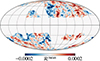 |
Fig. A.3. Similar to Fig A.2, but for the mean inferred adiabatic curvature fluctuation map. |
| In the text | |
|
Fig. A.4. Similar to Fig A.2, but for the uncertainty of the inferred adiabatic curvature fluctuation map. |
| In the text | |
|
Fig. A.5. Similar to Fig A.2, but for the residual adiabatic curvature fluctuation map, defined as ℛground truth − ℛmean inferred. |
| In the text | |
|
Fig. B.1. Correlation length of all chains, illustrating the rate at which samples in the various chains achieve independence. The typical correlation length for the chains is around 10 000 samples when bias parameters are also sampled. |
| In the text | |
|
Fig. B.2. Correlation matrix of Run #4 (the primary run). The correlation matrix illustrates the pairwise relationships among variables, with colour-coding indicating the strength and direction of correlations, aiding in the identification of patterns and dependencies within the dataset. The results show little to no correlation, except for a mild anti-correlation between fNL and the linear bias values. |
| In the text | |
|
Fig. B.3. Correlation matrix of Run #7 (which includes the sampling of the scale-dependent bias parameters, bϕ and bϕ, δ). Colour coding indicates the strength and direction of the correlations, illustrating the little to no correlation between fNL and the non-linear bias parameters, including the scale-dependent bias parameters. |
| In the text | |
|
Fig. B.4. Corner plot for fNL and bias parameters, for Run #4, catalogue 1. The corner plot displays the joint distributions and marginal distributions of the variables in the multidimensional dataset covered by fNL and the bias parameters. Each subplot captures the relationships between pairs of variables, offering an overview of the dataset structure and dependencies. For the main run, there are few to no degeneracies in the bias parameters. |
| In the text | |
|
Fig. B.5. Corner plot for fNL and bias parameters, for Run #4, catalogue 2. Similar to Fig. B.4, there are little to no degeneracies between fNL and the bias parameters. |
| In the text | |
|
Fig. B.6. Corner plot for fNL and bias parameters, for Run #4, catalogue 3. Similar to Fig. B.4, there are little to no degeneracies between fNL and the bias parameters. |
| In the text | |
|
Fig. B.7. Corner plot for fNL and bias parameters, for Run #4, catalogue 4. Similar to Fig. B.4, there are few to no degeneracies between fNL and the bias parameters. |
| In the text | |
|
Fig. B.8. Corner plot for fNL and bias parameters, for Run #7, catalogue 1. Similar to Fig. B.4, there are little to no degeneracies between fNL and the bias parameters. |
| In the text | |
|
Fig. B.9. Corner plot for fNL and bias parameters, for Run #7, catalogue 2. Similar to Fig. B.4, there are little to no degeneracies between fNL and the bias parameters. |
| In the text | |
|
Fig. B.10. Corner plot for fNL and bias parameters, for Run #7, catalogue 3. Similar to Fig. B.4, there are few to no degeneracies between fNL and the bias parameters. |
| In the text | |
|
Fig. B.11. Trace plots of the inferred values of fNL for the seven runs. Each panel shows the thinned chains, displaying only every 1, 000th sample, with the raw chain in red, the posterior mean in black (solid line), and the 1σ interval in gray (dashed lines). The last panel summarises the effective sample sizes (ESS) for all runs, which are computed for the entire, unthinned chain. All chains exhibit stable convergence around well-defined mean values, with sufficiently large ESS to ensure reliable inference. |
| In the text | |
|
Fig. C.1. Averaged projections of the mock data fields. The colour bar displays the number of galaxies in each pixel, which contains the sum of all galaxies in the summed-over axis. The image is intended to demonstrate the effects of the window function on the observed data and how the method can account for it. The galaxy field projected here is used for Run #4. Each pixel covers a width of 8000 h−1 Mpc/256 = 31.25 h−1 Mpc. |
| In the text | |
|
Fig. C.2. Averaged projections of the ground truth and statistical summaries of the inferred fields. The edge of the survey is highlighted with dotted lines, which means that voxels outside the edge are not observed. In the left panel, the ground truth density field is plotted. In the middle panel, the mean of the ensemble of the inferred fields is plotted. In the right panel, the standard deviation of the ensemble of the inferred fields is plotted. The image illustrates the method’s capability to recover the ground truth density field within the regions of observed data. We note that the voxels within the window selection function have less uncertainty and larger inferred means. The inferred fields are the product of Run #4. Each pixel covers a width and height of 8000 h−1 Mpc/256 = 31.25 h−1 Mpc. |
| In the text | |
Current usage metrics show cumulative count of Article Views (full-text article views including HTML views, PDF and ePub downloads, according to the available data) and Abstracts Views on Vision4Press platform.
Data correspond to usage on the plateform after 2015. The current usage metrics is available 48-96 hours after online publication and is updated daily on week days.
Initial download of the metrics may take a while.