


| Issue |
A&A
Volume 710, June 2026
|
|
|---|---|---|
| Article Number | L32 | |
| Number of page(s) | 8 | |
| Section | Letters to the Editor | |
| DOI | https://doi.org/10.1051/0004-6361/202659892 | |
| Published online | 23 June 2026 | |
Letter to the Editor
Magnetised CGM gas at z ∼ 1 revealed by SPICE-RACS
1
Departamento de Física de la Tierra y Astrofísica & IPARCOS-UCM, Universidad Complutense de Madrid, 28040 Madrid, Spain
2
SKA Observatory, SKA-Low Science Operations Centre, 26 Dick Perry Avenue, Kensington, WA 6151, Australia
3
ATNF, CSIRO Space & Astronomy, PO Box 1130 Bentley, WA 6102, Australia
4
Research School of Astronomy & Astrophysics, The Australian National University, Canberra, ACT 2611, Australia
5
Minnesota Institute for Astrophysics, University of Minnesota, 116 Church Street SE, Minneapolis, MN 55455, USA
6
Department of Astronomy and Astrophysics, University of California, Santa Cruz, 1156 High Street, Santa Cruz, CA 95069, USA
7
Dunlap Institute for Astronomy and Astrophysics, University of Toronto, 50 St. George Street, Toronto M5S 3H4, ON, Canada
8
David A. Dunlap Department of Astronomy and Astrophysics, University of Toronto, 50 St. George Street, Toronto M5S 3H4, ON, Canada
9
Max-Planck-Institut für Radioastronomie, Auf dem Hügel 69, 53121 Bonn, Germany
10
Mizusawa VLBI Observatory, National Astronomical Observatory of Japan, 2-21-1, Osawa, Mitaka, Tokyo 181-8588, Japan
11
Hamburg University, Hamburger Sternwarte, Gojenbergsweg 112, D-21029 Hamburg, Germany
12
INAF – Istituto di Radioastronomia, via P. Gobetti 101, 40129 Bologna, Italy
13
CSIRO Information Management & Technology, PO Box 883 Kenmore, QLD 4069, Australia
14
Department of Social Design Engineering, National Institute of Technology, Kochi College, 200-1 Monobe, Nankoku, Kochi 783-8508, Japan
★ Corresponding author: This email address is being protected from spambots. You need JavaScript enabled to view it.
Received:
16
March
2026
Accepted:
28
April
2026
Abstract
Magnetic fields are expected to permeate the circumgalactic medium (CGM) of galaxies, but direct constraints at high redshift remain limited by the lack of high-quality Faraday rotation measure (RM) data. Using the RMs from SPICE-RACS DR2 combined with the DESI DR1 quasar catalogue, we compiled the largest sample to date of 2483 quasar sightlines with associated RMs, including 612 with intervening Mg II absorbers tracing foreground galaxies and 1871 control sightlines without Mg II absorbers. After subtracting the Galactic RM contribution and restricting the analysis to sightlines with a low Milky Way H I column density and Hα intensity, we obtained a foreground-cleaned sample of 757 quasars (191 Mg II/566 control) spanning redshifts 0.13 < z < 3.45. In this foreground-cleaned sample, Mg II sightlines exhibit a 4.5σ excess in the residual RM dispersion of 4.13 ± 0.91 rad m−2 relative to the control sample at a median absorber redshift of z ∼ 1.14. This implies model-dependent CGM magnetic field strengths of ∼0.4 − 0.8 μG over projected radii of 20–150 kpc. This indicates that substantial CGM magnetisation was already established by z ∼ 1, enabling new constraints on the growth and amplification of magnetic fields in galaxy halos over cosmic time.
Key words: magnetic fields / galaxies: high-redshift / galaxies: magnetic fields
© The Authors 2026
 Open Access article, published by EDP Sciences, under the terms of the Creative Commons Attribution License (https://creativecommons.org/licenses/by/4.0), which permits unrestricted use, distribution, and reproduction in any medium, provided the original work is properly cited.
This article is published in open access under the Subscribe to Open model. This email address is being protected from spambots. You need JavaScript enabled to view it. to support open access publication.
1. Introduction
The circumgalactic medium (CGM) is a vast, multiphase reservoir of magnetised gas extending beyond galactic disks (Tumlinson et al. 2017). Magnetic fields in and around galaxies can affect the CGM dynamics by regulating gas cooling, cosmic-ray confinement, and angular momentum transport. Observations of polarised synchrotron emission and Faraday rotation reveal that coherent and turbulent magnetic fields extend beyond galactic disks. They are thought to trace outflows, inflows, and feedback-driven winds (Kronberg & Perry 1982; Kronberg et al. 2008; Bernet et al. 2008; Farnes et al. 2014; Prochaska & Zheng 2019; Ravi 2019; Shah & Seta 2021; Khrykin et al. 2026). It is therefore essential to characterise the strength, structure, and origin of magnetic fields in the CGM of high-redshift (z) galaxies for a complete understanding of galaxy evolution and cosmic magnetism.
While magnetic fields with strengths of a few μG are well established in galaxy disks and inner halos, their properties in the extended CGM (∼20–150 kpc) remain poorly constrained. Edge-on galaxy surveys such as Continuum Halos in Nearby Galaxies, an EVLA Survey (CHANG-ES), reveal ordered X-shaped halo fields and regular magnetic components within ∼5–15 kpc of galactic disks and discussed magnetised halos extending into the CGM (Wiegert et al. 2015). More direct probes are provided by Faraday rotation measures (RMs) from background radio sources, either as a function of impact parameter or through absorber-selected samples. Early studies of Mg II systems (Bernet et al. 2008, 2010; Kim et al. 2016) reported substantial RM excesses of ∼10 rad m−2 without accounting for Milky Way contamination, while subsequent investigations (Malik et al. 2020; Lan & Prochaska 2020), based on NRAO VLA Sky Survey (NVSS) RMs with large uncertainties and poorly constrained Galactic RM (GRM) modelling, inferred extragalactic RM signals implying ≳μG magnetic fields at tens of kiloparsecs. In contrast, modern RM grids, including recent analyses based on Low Frequency Array (LOFAR), found excesses of ≲4.0 rad m−2 that imply ≲μG field strengths within ∼50–100 kpc in low-z galaxies (Heesen et al. 2023). At z ∼ 0.5, lensed quasars have also been used to probe magnetic fields in the galaxy disks (Mao et al. 2017) and halos (Böckmann et al. 2023; Kovacs et al. 2026), while at z ∼ 2.6 Geach et al. (2023), de Roo et al. (2025) reported a high magnetic field of ∼500 μG in the molecular disk. Therefore, a detailed investigation is needed using large samples of precise RMs as these studies differ strongly.
In this Letter, we detect a statistically robust RM excess for Mg II-absorber galaxies by compiling a sample of high-precision RMs of quasars that is three times larger than previous studies, using observations obtained with the Australian SKA Pathfinder (ASKAP), to probe magnetised CGM environments at high redshift (z ∼ 1). To mitigate Milky Way contamination, we employed a bespoke annulus-based Galactic rotation measure (GRM) estimation method and removed sightlines passing through regions with a high gas density and ionisation in the Galactic foreground. This carefully filtered RM sample allowed us to better isolate the extragalactic signal and constrained the magnetisation of the CGM in Mg II-selected galaxies.
2. Data
For the RM measurements, we used the recently developed Spectra and Polarisation in Cutouts of Extragalactic Sources Rapid ASKAP Continuum Survey (SPICE-RACS1) Data Release 2, which covers the entire southern sky and extends up to a declination of +49° in the north (Thomson et al. 2026). The survey operates over a frequency range of 800–1088 MHz with an average angular resolution of ∼15″. With an rms noise of ∼200 μJy, approximately five million radio components are reported. By applying cuts of snr_polint > 8, fracpol > 0.005 and a flag as defined in DR2 based on poor convergence in fitting the Stokes I spectrum, stokesI_fit_flag2 < 5 and considering single RM components within 10″, a catalogue of ∼250 000 unique RM components were produced. This is the RM sample we used in our subsequent analysis.
To determine the RMs associated with quasars, we cross-matched the sources with the Dark Energy Spectroscopic Instrument (DESI) DR1 spectroscopic quasar catalogue (DESI Collaboration 2026). This catalogue contains ∼1.6 million sources up to a redshift of z ∼ 5.0, with a spectral resolution ranging from R ∼ 2000–5000 over the wavelength range 3000–9800 Å, and it provides a sub-arcsecond spatial resolution with a sky coverage of −18° < δ < +84°. The completeness within this coverage is not uniform (see Fig. 1).
 |
Fig. 1. All-sky map of the Galactic neutral hydrogen (H I) column density from the HI4PI survey, overlaid with the clean RRM sample (757 sources). Positive and negative RRMs are shown with red and blue circles, respectively, with the circle size proportional to |RRM|. The sky coverage of the sources is limited in declination by the SPICE-RACS upper limit of ∼ + 49°, and the lower limit of −18° is from DESI. In addition, the source scarcity in some low HI density regions is due to the patchy coverage in the DESI DR1 observations (see DESI Collaboration 2026, fig. 3, top panel). |
We cross-matched the SPICE-RACS and DESI catalogue positions using a matching radius of 3″, considering the angular resolutions of DESI and SPICE-RACS. This resulted in a sample of 2483 unique sources that are well characterised at the optical and radio wavelengths and have a Galactic latitude |b|> 20° (to minimise the contribution from the Galactic plane).
To classify the sightlines based on the presence of foreground galaxies, we used the Mg II doublet absorption lines at wavelengths λλ 2796 & 2803 Å detected in the quasar spectra (Napolitano et al. 2023). The presence of these absorbers is widely regarded as a reliable proxy for intervening foreground galaxies (Kacprzak et al. 2008; Chen et al. 2010). Some of the sightlines have more than one absorber along the line of sight. The RMs of the sightlines with and without Mg II absorbers were used to constrain the magnetised plasma in the CGM of these galaxies.
2.1. Removing the Milky Way RM contribution
To estimate the foreground GRM for each RM component, we adopted an annulus-based method (Anderson et al. 2024) that we discuss in Appendix A, and we obtained the residual RM defined as RRM = RM − GRM. In Fig. B we use the RM structure functions to show that the GRM subtraction using the annulus method effectively removes the majority of the scale-dependent GRM from the RM.
2.2. Clean RM sample selection using HI and Hα cuts
After correcting the RMs for the Milky Way contribution using the GRM, it is essential to further examine the potential residual contamination arising from the high-density regions of the interstellar medium. We found that the RRM dispersion is strongly correlated with H I (using the HI4PI map, HI4PI Collaboration 2016) and the Hα intensity (from the WHAM map, Haffner et al. 2003), as shown in Fig. C.2, indicating that the GRM is not removed completely. Therefore, the high-density warm ionised and neutral phases of the Milky Way, traced by Hα and H I emission, respectively, contribute to the excess scatter in the RRM values.
To minimise these effects and obtain a reliable set of sightlines, we selected sightlines with an H I column density and Hα intensity below 3.5 × 1020 cm−2 and 1 Rayleigh (R), respectively (for details, see Appendix C). Application of these cuts yielded the final clean sample of 757 sources over redshifts 0.13 < z < 3.45 (as shown in Fig. 1). It includes 191 and 566 sightlines with and without Mg II absorbers, respectively (see Fig. C.5 for the redshift distribution). This sample represents a minimally contaminated set of sightlines for probing the extragalactic RM signal and for assessing the contribution of intervening Mg II absorbers to the observed RRM dispersion.
3. Results
3.1. RRM excess in Mg II absorbers
To demonstrate the statistical difference between the RRM distributions of the subsamples with and without Mg II absorbers, we plot the cumulative distribution function (CDF) of |RRM| in Fig. 2. The CDF clearly shows a systematic shift towards higher RRM values for the Mg II absorber subsample. To quantify the RM contribution of the foreground Mg II absorbers in the redshift range of 0.39 < z < 2.32, we computed the excess RRM dispersion associated with the Mg II absorbers as
 (1)
(1)
 |
Fig. 2. Cumulative distribution function of |RRM| for the subsamples with and without foreground Mg II absorbers. |
where σMAD, MgII and σMAD, noMgII represent the median absolute deviation of RRM for the subsamples with and without Mg II absorbers, respectively. The uncertainties were propagated to RRM from RM and GRM, and further uncertainties on σMAD of each sample by taking rms of σMAD of simulating 103 realisations of the dataset. The results are summarised in Table 1. An excess RRM dispersion of 4.13 ± 0.91 rad m−2 at 4.5σ was found (the uncertainty was calculated using the equation in the footnote)3. For the sample with N = 1, we note that the excess is 5.22 ± 0.90 rad m−2, which is higher (∼1 rad m−2) than the value for the sample with N > 0. This requires further investigation. This RRM excess is comparable to that found by Heesen et al. (2023) for nearby galaxies using the high-precision LOFAR RMs (O’Sullivan et al. 2023). We note that the excess in the total sample before applying the HI and Hα cuts is statistically insignificant, with a value of 1.73 ± 1.65 rad m−2 (1σ).
RRM dispersion (σMAD) and excess for Mg II subsamples after all selection criteria.
We further tested the significance of the RRM excess by randomly drawing multiple subsamples of 191 sources from the non-absorber sample. The resulting excess has a median value of σexcess of 4.18 ± 1.06 rad m−2 with a range of 3.56 ± 1.3 to 5.36 ± 0.76 rad m−2. In Fig. 3 we show that the RRM excess is insensitive to the exact H I and Hα cuts, where the excess remains across a wide range of values. This is also true for the significance of the excess (Fig. C.3).
 |
Fig. 3. Map of the RRM excess for various cutoff limits of H I column density and Hα intensities to illustrate the variation of σExcess. We retained excess values when both subsamples (with and without Mg II absorbers) contained a minimum of 100 sightlines. The vertical green and horizontal blue lines mark the thresholds H I = 3.5 × 1020 cm−2 and Hα = 1.0 R, respectively, which we adopted to compute the values reported in the Table 1. The statistical significance heat map is shown in Fig. C.3. |
We also performed a Bayesian model comparison of the RRM to test whether sightlines with Mg II absorbers exhibit excess RM relative to the non-Mg II subsample. Assuming that the RRMs are Gaussian-distributed with zero mean, we modelled the observed scatter as the quadrature sum of the measurement uncertainties and a dispersion, characterised using the Gaussian-equivalent σMAD. Two hypotheses were considered: H0, in which the Mg II and non-Mg II sightlines have a similar dispersion, and H1, in which the two samples have different dispersions. Adopting Jefferys priors on the dispersion parameters and marginalising over them, we computed the Bayesian evidence for both hypotheses and evaluated the Bayes factor. We found a Bayes factor of 41.6, providing very strong (decisive) evidence that the sample with Mg II has an RRM excess. In Appendix E we show that the RRM excess is not significantly affected when the sample is split by the radio spectral index (which was used by previous studies as a proxy for the source compactness).
3.2. Estimate of the magnetic field strength
To infer the physical CGM magnetic field, we simultaneously combined (i) the energy equipartition between the thermal gas and magnetic field and (ii) a turbulent Faraday-screen model for the RM dispersion. We assumed approximate pressure balance in the CGM,  . Here, ntot and T are the total gas density (hydrogen and helium) and temperature of the CGM, respectively. We related the electron density to the total gas density through an ionisation fraction xe such that ne = xentot. Adopting xe = 0.8 and T = 104 K (as appropriate for predominantly photoionised cool CGM gas; see Dutta et al. 2024), we obtained
  .
.
We modelled the Faraday rotation as arising from a turbulent magnetised plasma, for which the RM dispersion is given by (Gaensler et al. 2001; Seta & Federrath 2021)
 (2)
(2)
where B denotes the turbulent magnetic field strength, L is the CGM path length, l is the correlation length, and z is the absorber redshift. Substituting the equipartition relation ne(B) into the above equation, we solved for the magnetic field as a function of CGM path length, B(L), for a fixed observed excess σRM. We adopted l = L/10, and marginalised over the absorber redshift range z = 0.37 to 2.3 using a Monte Carlo approach with 103 samples.
For a plausible impact parameter of the line of sight and CGM extent of L = 20 − 150 kpc, we inferred magnetic field strength ranges B ≈ 0.4 to 0.8 μG. This corresponds to equipartition electron densities of ≈10−2 cm−3 to 10−3 cm−3. It is also possible that the CGM has a higher temperature and a relatively low ionisation fraction, which would result in lower ne.
4. Discussion and summary
The excess RRM detection in high-z Mg II absorbers provides robust evidence for magnetised gas in the CGM that might results from galactic outflows preferentially aligned with the host galaxy minor axis (Heesen et al. 2023). Several previous studies (Bernet et al. 2008; Farnes et al. 2014; Kim et al. 2016) have used RM measurements to infer magnetic fields in absorbers, but their results were severely affected by GRM contamination. Subsequent attempts (Basu et al. 2018; Malik et al. 2020; Lan & Prochaska 2020; Shah & Seta 2021; Heesen et al. 2023; Burman et al. 2024) used RRMs, with GRM subtractions based on relatively simplistic or incomplete foreground modelling. This left several discrepancies related to the large uncertainties of NVSS RMs, limited sample sizes, and incomplete treatment of Galactic foregrounds. We used RM measurements that are an order of magnitude more precise than NVSS, with a sample size approximately three times larger, and with significantly improved radio–optical positional matching. Moreover, we subtracted the GRM using an improved annulus-based method and excluded sightlines intersecting dense neutral and ionised Galactic regions, yielding a substantially more robust RRM sample. We found that the RRM excess in Mg II absorbers is significant, and this implies that normal galaxies host a magnetised CGM that is larger than predicted by simulations (e.g. Ramesh et al. 2023).
Several caveats remain in translating the observed RRM dispersion into physical magnetic field strengths. Conversions like this depend on poorly constrained CGM properties, including electron density, path length, and magnetic field coherence, which may vary substantially with halo mass, redshift, and environment. The residual Galactic RM structure, despite stringent H I and Hα cuts, may still contribute to the scatter, while source-dependent effects such as Faraday depolarisation can modulate the observed RRM independently of the intervening medium. Moreover, Mg II-selected absorbers preferentially trace cool metal-enriched gas and may not be representative of the full CGM volume. This might bias magnetic field estimates towards denser or more strongly magnetised regions. The estimates in Section 3.1 are affected by this, and a more detailed investigation of the radial variation and redshift evolution of the magnetic field in these absorbers will be presented in a follow-up paper.
Despite these limitations, this analysis used a conservative and homogeneous method and successfully isolated the extragalactic RM signal. In summary,
-
We compiled a sample of 2483 quasars with well-characterised radio and optical properties, extending up to z ∼ 4.0, of which 757 sightlines (191 with and 566 without Mg II) had a low foreground Galactic HI density and Hα intensity. We found a decisive (Bayes factor of ∼42) excess extragalactic RM associated with the Mg II absorbers of 4.13 ± 0.91 rad m−2 (4.5σ).
-
We emphasise that it is insufficient to mitigate Galactic contamination by GRM removal alone. Additional cuts of H I < 3.5 × 1020 cm−2 and Hα intensity < 1 R were needed to minimise the Milky Way RM contamination from dense and highly ionised regions, without which the RRM excess is not statistically significant (< 1σ).
-
We estimated the CGM magnetic field B ∼ 0.4 − 0.8 μG strength at typical radii between 20 to 150 kpc, assuming energy equipartition and nominal parameter values that require further detailed investigation.
This study provides a reliable assessment of CGM magnetisation at high-z and establishes a framework that is readily extendable to forthcoming high-density RM grids from the Polarisation Sky Survey of the Universe’s Magnetism (Gaensler et al. 2025) and the SKA, which will be essential for resolving the coherence scale, geometry, and redshift evolution of magnetic fields in the CGM.
References
- Anderson, C. S., McClure-Griffiths, N. M., Rudnick, L., et al. 2024, MNRAS, 533, 4068 [NASA ADS] [CrossRef] [Google Scholar]
- Basu, A., Mao, S. A., Fletcher, A., et al. 2018, MNRAS, 477, 2528 [NASA ADS] [CrossRef] [Google Scholar]
- Bernet, M. L., Miniati, F., Lilly, S. J., Kronberg, P. P., & Dessauges-Zavadsky, M. 2008, Nature, 454, 302 [NASA ADS] [CrossRef] [Google Scholar]
- Bernet, M. L., Miniati, F., & Lilly, S. J. 2010, ApJ, 711, 380 [NASA ADS] [CrossRef] [Google Scholar]
- Böckmann, K., Brüggen, M., Heesen, V., et al. 2023, A&A, 678, A56 [NASA ADS] [CrossRef] [EDP Sciences] [Google Scholar]
- Burman, S., Sharma, P., Malik, S., & Singh, S. 2024, JCAP, 2024, 063 [Google Scholar]
- Chen, H.-W., Helsby, J. E., Gauthier, J.-R., et al. 2010, ApJ, 714, 1521 [NASA ADS] [CrossRef] [Google Scholar]
- de Roo, W., Vegetti, S., Powell, D. M., et al. 2025, MNRAS, 540, L78 [Google Scholar]
- DESI Collaboration (Abdul Karim, M., et al.) 2026, AJ, 171, 285 [Google Scholar]
- Dutta, A., Bisht, M. S., Sharma, P., et al. 2024, MNRAS, 531, 5117 [Google Scholar]
- Farnes, J. S., O’Sullivan, S. P., Corrigan, M. E., & Gaensler, B. M. 2014, ApJ, 795, 63 [NASA ADS] [CrossRef] [Google Scholar]
- Gaensler, B. M., Dickey, J. M., McClure-Griffiths, N. M., et al. 2001, ApJ, 549, 959 [Google Scholar]
- Gaensler, B. M., Heald, G. H., McClure-Griffiths, N. M., et al. 2025, PASA, 42 [Google Scholar]
- Geach, J. E., Lopez-Rodriguez, E., Doherty, M. J., et al. 2023, Nature, 621, 483 [NASA ADS] [CrossRef] [Google Scholar]
- Haffner, L. M., Reynolds, R. J., Tufte, S. L., et al. 2003, ApJS, 149, 405 [NASA ADS] [CrossRef] [Google Scholar]
- Heesen, V., OSullivan, S. P., Brüggen, M., et al. 2023, A&A, 670, L23 [NASA ADS] [CrossRef] [EDP Sciences] [Google Scholar]
- HI4PI Collaboration (Ben Bekhti, N., et al.) 2016, A&A, 594, A116 [NASA ADS] [CrossRef] [EDP Sciences] [Google Scholar]
- Hutschenreuter, S., Anderson, C. S., Betti, S., et al. 2022, A&A, 657, A43 [NASA ADS] [CrossRef] [EDP Sciences] [Google Scholar]
- Kacprzak, G. G., Churchill, C. W., Steidel, C. C., & Murphy, M. T. 2008, AJ, 135, 922 [NASA ADS] [CrossRef] [Google Scholar]
- Khrykin, I. S., Tejos, N., Xavier Prochaska, J., et al. 2026, A&A, 706, A11 [NASA ADS] [CrossRef] [EDP Sciences] [Google Scholar]
- Kim, K. S., Lilly, S. J., Miniati, F., et al. 2016, ApJ, 829, 133 [NASA ADS] [CrossRef] [Google Scholar]
- Kovacs, T. O., Mao, S. A., Basu, A., Ma, Y. K., & Gaensler, B. M. 2026, A&A, 705, A28 [NASA ADS] [CrossRef] [EDP Sciences] [Google Scholar]
- Kronberg, P. P., & Perry, J. J. 1982, ApJ, 263, 518 [NASA ADS] [CrossRef] [Google Scholar]
- Kronberg, P. P., Bernet, M. L., Miniati, F., et al. 2008, ApJ, 676, 70 [CrossRef] [Google Scholar]
- Lan, T.-W., & Prochaska, J. X. 2020, MNRAS, 496, 3142 [CrossRef] [Google Scholar]
- Malik, S., Chand, H., & Seshadri, T. R. 2020, ApJ, 890, 132 [NASA ADS] [CrossRef] [Google Scholar]
- Mao, S. A., Carilli, C., Gaensler, B. M., et al. 2017, Nat. Astron., 1, 621 [NASA ADS] [CrossRef] [Google Scholar]
- Napolitano, L., Pandey, A., Myers, A. D., et al. 2023, AJ, 166, 99 [NASA ADS] [CrossRef] [Google Scholar]
- O’Sullivan, S. P., Shimwell, T. W., Hardcastle, M. J., et al. 2023, MNRAS, 519, 5723 [CrossRef] [Google Scholar]
- Planck Collaboration VI. 2020, A&A, 641, A6 [NASA ADS] [CrossRef] [EDP Sciences] [Google Scholar]
- Prochaska, J. X., & Zheng, Y. 2019, MNRAS, 485, 685 [Google Scholar]
- Ramesh, R., Nelson, D., Heesen, V., & Brüggen, M. 2023, MNRAS, 526, 5483 [NASA ADS] [CrossRef] [Google Scholar]
- Ravi, V. 2019, ApJ, 872, 88 [NASA ADS] [CrossRef] [Google Scholar]
- Seta, A., & Federrath, C. 2021, MNRAS, 502, 2220 [NASA ADS] [CrossRef] [Google Scholar]
- Shah, H., & Seta, A. 2021, MNRAS, 508, 1371 [NASA ADS] [CrossRef] [Google Scholar]
- Thomson, A. J. M., Galvin, T. J., Duchesne, S. W., et al. 2026, arXiv e-prints [arXiv:2605.16917] [Google Scholar]
- Tumlinson, J., Peeples, M. S., & Werk, J. K. 2017, ARA&A, 55, 389 [Google Scholar]
- Wiegert, T., Irwin, J., Miskolczi, A., et al. 2015, AJ, 150, 81 [Google Scholar]
SPICE–RACS is a joint initiative of the POSSUM Collaboration (possum-survey.org) and the ASKAP Observatory.
 .
.
Appendix A: GRM using annulus method and comparison with standard GRM Map
To estimate the foreground GRM for each RM component, we adopt an annulus-based method (Anderson et al. 2024). For each target source, we construct an annulus centered on its position with an inner radius of rinner = 0.2° (at z = 1.0, this corresponds to ∼5.9 Mpc using Planck cosmology (Planck Collaboration VI 2020)), to avoid both self-contamination and contamination from the CGM of the foreground galaxies, and then select the 20 nearest RMs from the full sample. To minimise the influence of outliers, we discard RMs exceeding 5σRM, where σRM is the standard deviation of the selected 20 RMs, and assign their median value as the GRM at that location. The GRM uncertainty is estimated as  , where σMAD is the median absolute deviation–based standard deviation and N = 20 (i.e. the statistical uncertainty).
To validate our GRM estimation procedure, we compare our locally derived Galactic RM values with the all-sky Galactic RM map of Hutschenreuter et al. (2022), which is based on a Information Field Theory reconstruction of extragalactic RM measurements. In the top panel of Fig. A.1, we show the GRM estimated from our annular method plotted against the corresponding GRM values extracted from their map at the same sky positions. They closely follow each other, with a few outliers and a near-unity slope, demonstrating that our local annulus-based approach reliably recovers the GRM from the Milky Way.
 |
Fig. A.1. Comparison of GRM values (top panel) and their associated uncertainties (bottom panel) for all sightlines in our sample, derived using the (Hutschenreuter et al. 2022) map and our bespoke annulus-based method. The red-dashed line shows the one-to-one relation. |
The bottom panel of Fig. compares the associated GRM uncertainties from our method with the uncertainty estimates provided by the Hutschenreuter et al. (2022) map. We can clearly see that the uncertainty from the (Hutschenreuter et al. 2022) method is larger than the annulus method (∼3 times on average). This behaviour is expected, as their map represents a smoothed Galactic foreground model with a lower spatial sampling of input data points than we have used. Therefore, we use the annulus method in our analysis, and the resulting RRMs are not dominated by foreground systematics. The histogram shown in Fig. A.2 also highlights the same.
 |
Fig. A.2. Histograms of RM (blue) and RRM (orange) for all sightlines in the sample show the impact of the GRM. We have also overplotted the RRM (clean sample after cuts, green) to show the impact of HI and Hα cuts. |
Appendix B: Structure function Analysis
To assess the impact of GRM removal on the RM, we computed the two-point structure function for both the RM and RRM using the full sample, prior to applying any H I or Hα threshold criteria. The resulting structure functions are shown in Fig. B.1. A direct comparison between the RM and RRM structure functions highlights that the majority of the scale-dependent GRM contributions are removed; however, at scales smaller than ∼0.7°, their effects remain.
 |
Fig. B.1. Structure function of RM as a function of angular separation (left panel), for RRM (right panel). |
Appendix C: HI and Hα threshold
In Fig. C.1, we overlay the full sample of sightlines on the HI4PI H I column density map using the HI4PI map from HI4PI Collaboration (2016) (in the left panel) and Hα intensity using Wisconsin H-Alpha Mapper (WHAM4; Haffner et al. 2003) (in the right panel) to visually assess the correspondence between the neutral and ionised gas distribution and the observed RRMs. The full sample RRMs are shown as red (positive) and blue (negative) circles, with the circle size representing the absolute value of the RRM. We note that a subset of sightlines passes through high–neutral and ionised regions, which are likely to host stronger magnetic fields and can therefore have a significant impact on the measured RMs.
 |
Fig. C.1. Left panel: All-sky map of HI column density, overlaid with the full sample RRM (+ve with red circle and −ve with blue circle), where circle size indicates the |RRM|. Right panel: Same as left but with Hα intensity in the background. |
To investigate the impact of high H I column density and Hα regions on our analysis, we analysed the H I and Hα intensity from the HI4PI and WHAM survey for each line of sight in our sample. We then computed the σMAD of RRM (combined sample of with and without Mg II systems) as a function of H I column density and Hα intensity, using sources below the different cutoffs, as shown in Fig. C.2. The resulting trends show a clear increase in σMAD with increasing NH I and Hα intensity, indicating that regions with high neutral and ionised gas density exhibit significantly enhanced Faraday dispersion. This increase of σMAD (even though only 15% from lowest to highest values) is significant enough to affect the analysis. In particular, it can affect the excess results and their uncertainty. These results demonstrate that high–H I and Hα regions can substantially contaminate the extragalactic RM signal, motivating the need for an H I and Hα-based threshold in our analysis. We have estimated the RRM excess map as shown Section 3.1 and its significance map is shown in Fig. C.3.
 |
Fig. C.2. Map of the σMAD of RRM for various H I column density and Hα intensity cutoffs for the total clean sample with and without Mg II absorbers. For each cutoff in both axes, a minimum of 100 Mg II sightlines is required, leading to missing pixels at low Hα and H I. The vertical green and horizontal blue lines mark the thresholds NHI = 3.5 × 1020 cm−2 and Hα = 1.0 R, respectively. |
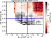 |
Fig. C.3. Map of the statistical significance of RRM excess shown in Fig. 3 for various H I column density and Hα intensity cutoff. |
To determine an appropriate cutoff, we examined the GRM uncertainty as a function of H I column density and Hα intensity for the full sample, as shown in Fig. C.4. We find that the GRM uncertainty increases systematically with increasing H I density and Hα intensity. To retain sightlines with relatively low GRM uncertainty, we impose H I and Hα thresholds at which the GRM uncertainty falls below the mean uncertainty of the full sample. This yields a cutoff of NHI = 3.5 × 1020cm−2, and Hα = 1 R ( ), resulting in a reduced sample of 757 sightlines. This selection minimises contamination from turbulent or multiphase Galactic regions and enables a more robust interpretation of the extragalactic RRM statistics.
 |
Fig. C.4. The GRM error plotted against H I column density (bottom x-axis), and Hα intensity (top x-axis). Vertical dashed red and dotted blue lines mark the H I and Hα thresholds, respectively. |
 |
Fig. C.5. Histogram of the quasars’ redshift for the clean subsamples with and without Mg II absorbers, along with the redshift of the Mg II absorbers. |
Appendix D: HI and Hα correlation
As shown in the Appendix C, high-density neutral and ionised regions, quantified by H I column density and Hα intensity, have a significant impact on our analysis. We also examined the one-to-one correlation between H I and Hα intensity and present the corresponding scatter plot in Fig. D.1. As seen, these two quantities do exhibit a mild one-to-one correlation. Therefore, to minimise their impact on our analysis, we apply both cutoffs to filter the sightlines, as discussed in Section 2.2. We have also plotted the histogram of Galactic latitude for the clean sample in Fig. D.2. We note that most sources lie at high Galactic latitudes, indicating minimal contamination from the Galactic plane in our analysis.
 |
Fig. D.1. Distribution of H I column density and Hα intensity for the full sample. The dashed vertical and horizontal lines indicate the adopted thresholds. The clean sample is represented by sources lying below both cutoffs. |
 |
Fig. D.2. Histogram of Galactic latitude of the clean sample. All these sources have |b|> 20°. |
Appendix E: Classification based on Spectral Indices
The optical and radio observations originate from different telescopes with differing angular resolutions, and therefore the observed source extents may not be perfectly aligned. The radio spectral indices, α (Sν ∝ να), provide information on the compactness of the quasars, which serves as an indicator of the alignment between the radio and optical sightlines. Accordingly, we divided the sample into three spectral categories based on the radio spectral index from Thomson et al. (2026): steep (α < −0.6), typically associated with extended sources; flat (α ≥ −0.4), generally core-dominated; and mid-spectrum (−0.6 < α ≤ −0.4). For each category, we evaluated the σMAD of the RRM separately for sightlines with and without foreground Mg II absorbers. The results are summarised in Table E.1.
RRM dispersion (σMAD) and excess for Mg II subsamples by spectral type.
We find that the RRM excess in the subsample with Mg II absorbers is present in both the steep- and flat-spectrum sources, which is contrary to the earlier findings of Malik et al. (2020). In that work, the RRM excess associated with foreground Mg II absorbers was reported only for core-dominated sources. However, due to the relatively low resolution of the radio and optical data used in that study, the positional association was limited to a separation of ∼7″, which may have affected the morphological classification. With the advent of high-resolution optical data from DESI and radio data from ASKAP, the positional separation between radio and optical counterparts is reduced to ∼3″, allowing more reliable associations. As a result, we now find that sightlines classified as steep-spectrum sources, which were previously considered to arise from extended emission regions, may also lie close to optical counterparts and thus pass through foreground galaxies. This further strengthens the evidence for magnetised plasma in the halos of intervening galaxies.
Appendix F: Acknowledgements
We thank the anonymous referee for constructive comments that significantly improved the paper. SM, SPO and DAL acknowledge support from grant PID2023-146372OB-I00, funded by MICIU/AEI/10.13039/501100011033 and by ERDF, EU. SPO acknowledge support from the Comunidad de Madrid Atracción de Talento program via grant 2022-T1/TIC-23797. C.S.A. acknowledges funding from the Australian Research Council in the form of Australian Future Fellowship FT240100498. AS is supported by the Australian Research Council through the Discovery Early Career Researcher Award (DECRA) Fellowship (project DE250100003) funded by the Australian Government and the Australia-Germany Joint Research Cooperation Scheme of Universities Australia (UA–DAAD, 2025–2026).
This scientific work uses data obtained from Inyarrimanha Ilgari Bundara / the Murchison Radio-astronomy Observatory. We acknowledge the Wajarri Yamaji People as the Traditional Owners and native title holders of the Observatory site. The Australian SKA Pathfinder is part of the Australia Telescope National Facility (https://ror.org/05qajvd42) which is managed by CSIRO. Operation of ASKAP is funded by the Australian Government with support from the National Collaborative Research Infrastructure Strategy. ASKAP uses the resources of the Pawsey Supercomputing Centre. Establishment of ASKAP, the Murchison Radio-astronomy Observatory and the Pawsey Supercomputing Centre are initiatives of the Australian Government, with support from the Government of Western Australia and the Science and Industry Endowment Fund.
This research used data obtained with the Dark Energy Spectroscopic Instrument (DESI). DESI construction and operations is managed by the Lawrence Berkeley National Laboratory. This material is based upon work supported by the U.S. Department of Energy, Office of Science, Office of High-Energy Physics, under Contract No. DE–AC02–05CH11231, and by the National Energy Research Scientific Computing Center, a DOE Office of Science User Facility under the same contract. Additional support for DESI was provided by the U.S. National Science Foundation (NSF), Division of Astronomical Sciences under Contract No. AST-0950945 to the NSF’s National Optical-Infrared Astronomy Research Laboratory; the Science and Technology Facilities Council of the United Kingdom; the Gordon and Betty Moore Foundation; the Heising-Simons Foundation; the French Alternative Energies and Atomic Energy Commission (CEA); the National Council of Humanities, Science and Technology of Mexico (CONAHCYT); the Ministry of Science and Innovation of Spain (MICINN), and by the DESI Member Institutions: www.desi.lbl.gov/collaborating-institutions. The DESI collaboration is honored to be permitted to conduct scientific research on I’oligam Du’ag (Kitt Peak), a mountain with particular significance to the Tohono O’odham Nation. Any opinions, findings, and conclusions or recommendations expressed in this material are those of the author(s) and do not necessarily reflect the views of the U.S. National Science Foundation, the U.S. Department of Energy, or any of the listed funding agencies.
All Tables
RRM dispersion (σMAD) and excess for Mg II subsamples after all selection criteria.
All Figures
|
Fig. 1. All-sky map of the Galactic neutral hydrogen (H I) column density from the HI4PI survey, overlaid with the clean RRM sample (757 sources). Positive and negative RRMs are shown with red and blue circles, respectively, with the circle size proportional to |RRM|. The sky coverage of the sources is limited in declination by the SPICE-RACS upper limit of ∼ + 49°, and the lower limit of −18° is from DESI. In addition, the source scarcity in some low HI density regions is due to the patchy coverage in the DESI DR1 observations (see DESI Collaboration 2026, fig. 3, top panel). |
| In the text | |
|
Fig. 2. Cumulative distribution function of |RRM| for the subsamples with and without foreground Mg II absorbers. |
| In the text | |
|
Fig. 3. Map of the RRM excess for various cutoff limits of H I column density and Hα intensities to illustrate the variation of σExcess. We retained excess values when both subsamples (with and without Mg II absorbers) contained a minimum of 100 sightlines. The vertical green and horizontal blue lines mark the thresholds H I = 3.5 × 1020 cm−2 and Hα = 1.0 R, respectively, which we adopted to compute the values reported in the Table 1. The statistical significance heat map is shown in Fig. C.3. |
| In the text | |
|
Fig. A.1. Comparison of GRM values (top panel) and their associated uncertainties (bottom panel) for all sightlines in our sample, derived using the (Hutschenreuter et al. 2022) map and our bespoke annulus-based method. The red-dashed line shows the one-to-one relation. |
| In the text | |
|
Fig. A.2. Histograms of RM (blue) and RRM (orange) for all sightlines in the sample show the impact of the GRM. We have also overplotted the RRM (clean sample after cuts, green) to show the impact of HI and Hα cuts. |
| In the text | |
|
Fig. B.1. Structure function of RM as a function of angular separation (left panel), for RRM (right panel). |
| In the text | |
|
Fig. C.1. Left panel: All-sky map of HI column density, overlaid with the full sample RRM (+ve with red circle and −ve with blue circle), where circle size indicates the |RRM|. Right panel: Same as left but with Hα intensity in the background. |
| In the text | |
|
Fig. C.2. Map of the σMAD of RRM for various H I column density and Hα intensity cutoffs for the total clean sample with and without Mg II absorbers. For each cutoff in both axes, a minimum of 100 Mg II sightlines is required, leading to missing pixels at low Hα and H I. The vertical green and horizontal blue lines mark the thresholds NHI = 3.5 × 1020 cm−2 and Hα = 1.0 R, respectively. |
| In the text | |
|
Fig. C.3. Map of the statistical significance of RRM excess shown in Fig. 3 for various H I column density and Hα intensity cutoff. |
| In the text | |
|
Fig. C.4. The GRM error plotted against H I column density (bottom x-axis), and Hα intensity (top x-axis). Vertical dashed red and dotted blue lines mark the H I and Hα thresholds, respectively. |
| In the text | |
|
Fig. C.5. Histogram of the quasars’ redshift for the clean subsamples with and without Mg II absorbers, along with the redshift of the Mg II absorbers. |
| In the text | |
|
Fig. D.1. Distribution of H I column density and Hα intensity for the full sample. The dashed vertical and horizontal lines indicate the adopted thresholds. The clean sample is represented by sources lying below both cutoffs. |
| In the text | |
|
Fig. D.2. Histogram of Galactic latitude of the clean sample. All these sources have |b|> 20°. |
| In the text | |
Current usage metrics show cumulative count of Article Views (full-text article views including HTML views, PDF and ePub downloads, according to the available data) and Abstracts Views on Vision4Press platform.
Data correspond to usage on the plateform after 2015. The current usage metrics is available 48-96 hours after online publication and is updated daily on week days.
Initial download of the metrics may take a while.