


| Issue |
A&A
Volume 710, June 2026
|
|
|---|---|---|
| Article Number | A325 | |
| Number of page(s) | 13 | |
| Section | Stellar structure and evolution | |
| DOI | https://doi.org/10.1051/0004-6361/202659792 | |
| Published online | 24 June 2026 | |
Discovery of the first octupole pulsation mode in a δ Scuti star
A stationary ℓ= 3 sectoral mode
1
HUN–REN–SZTE Stellar Astrophysics Research Group, H-6500 Baja, Szegedi út, Kt. 766, Hungary
2
Department of Physics, Kavli Institute for Astrophysics and Space Research, M.I.T., Cambridge, MA 02139, USA
3
Department of Astronomy, Cornell University, 122 Sciences Dr, Ithaca, NY 14850, USA
4
Nicolaus Copernicus Astronomical Center, Polish Academy of Sciences, ul. Bartycka 18, PL-00-716 Warszawa, Poland
5
Centre for Space Research, North-West University, Mahikeng 2745, South Africa
6
Jeremiah Horrocks Institute, University of Lancashire, Preston PR1 2HE, UK
7
Harvard University, Cambridge, MA 02138, USA
8
Amateur Astronomer, Glendale, AZ 85308, USA
9
NASA Goddard Space Flight Center, 8800 Greenbelt Road, Greenbelt, MD 20771, USA
10
TAPIR, Mailcode 350-17, California Institute of Technology, Pasadena, CA 91125, USA
11
Baja Astronomical Observatory of University of Szeged, H-6500 Baja, Szegedi út, Kt. 766, Hungary
12
Konkoly Observatory, Research Centre for Astronomy and Earth Sciences, H-1121 Budapest, Konkoly, Thege Miklós út 15-17, Hungary
13
ELTE Eötvös Loránd University, Gothard Astrophysical Observatory, Szent Imre h. u. 112, 9700 Szombathely, Hungary
14
HUN–REN–ELTE Exoplanet Research Group, H-9700 Szombathely, Szent Imre h. u. 112, Hungary
15
SETI Institute, 189 Bernardo Avenue, Suite 200 Mountain View, CA 94043, USA
16
Astronomical Institute of the Wrocław University, ul. Kopernika 11, 51-622 Wrocław, Poland
17
Copernicus Astronomical Center, Bartycka 18, 00-716 Warsaw, Poland
★ Corresponding authors: This email address is being protected from spambots. You need JavaScript enabled to view it.
; This email address is being protected from spambots. You need JavaScript enabled to view it.
Received:
11
March
2026
Accepted:
17
April
2026
Abstract
Aims. We attempt to understand better how stellar pulsations in close binary systems are affected, and possibly induced, by tidal, Coriolis, and centrifugal forces.
Methods. We analyzed TESS data for some 50 000 potential eclipsing binaries selected by machine-learning algorithms in order to search for pulsation multiplets split by integer multiples of the orbital frequency.
Results. We report the discovery of an octupole pulsation mode in the binary star system TIC 287869463. The star system contains a δ Scuti star. This mode is actually a combination of Y3 + 3 and Y3 − 3 modes that are perturbed into a new eigenmode of the star via tidal, Coriolis, and centrifugal forces, which we call a Y33+ mode. The mode is stationary on the star, as opposed to being a traveling wave around the pulsation equator. To our knowledge, this is the first time that such an ℓ = 3 mode identification has been securely made in any δ Scuti star, and it is the first stationary ℓ = 3 sectoral mode of this type seen in any star, including the Sun. The ℓ = 3 pulsations appear as a combination of two components at 34.94617 d−1 and 39.31127 d−1, split by exactly six times the frequency of the orbital motion to within better than 1 part in 105. We extracted the pulsation frequencies from the TESS data spanning more than three years and modeled the system to gain a better understanding of this novel asteroseismic discovery. The pulsation frequencies are found to steadily increase with time, but they always maintain a split equal to six times the orbital frequency.
Conclusions. We discuss the implications for the broader class of tidally tilted pulsators and triaxial pulsators that have been discovered to date. We conclude that these previous categories can all be interpreted as linear combinations of spherical harmonics whose axes coincide with the orbital axis and form new eigenmodes of the star via tidal, Coriolis, and centrifugal perturbations
Key words: binaries: eclipsing / binaries: general / stars: interiors / stars: oscillations
© The Authors 2026
 Open Access article, published by EDP Sciences, under the terms of the Creative Commons Attribution License (https://creativecommons.org/licenses/by/4.0), which permits unrestricted use, distribution, and reproduction in any medium, provided the original work is properly cited.
This article is published in open access under the Subscribe to Open model. This email address is being protected from spambots. You need JavaScript enabled to view it. to support open access publication.
1. Introduction
Stellar pulsations have been studied for more than a century since 1919, when Eddington began to explore the theory of stellar pulsation with particular interest in understanding Cepheid variables (Eddington 1919a,b, 1926). For the first half-century of the study of stellar pulsation, it was assumed that the surface geometry of pulsation modes could be described adequately by spherical harmonics (Cowling 1941), which are the eigenmode solutions to pulsation equations for perfectly spherical stars. The geometry of eigenmodes associated with the spherical harmonics is described by three quantum numbers: n, the radial overtone, which is the number of radial nodes that are spherical shells; ℓ, the degree, which is the number of surface nodes of the mode; and m, the azimuthal order, which gives the number of surface nodes that are lines of longitude. It was further assumed that the axis of pulsation coincided with the rotation axis of all pulsating stars, since that, in most cases, is the principal axis of distortion from spherical symmetry (see, e.g., Kurtz 2022 and Aerts et al. 2010 for reviews).
Traditionally, in stars other than the Sun, the degree of the mode is inferred, rather than observed directly. Surface cancellation of observed sectors of the spherical harmonics has meant that modes of higher degree (ℓ ≥ 3) have been difficult to detect, since these higher-degree modes have very low visibility (Dziembowski 1977). On the other hand, because the Sun has a well-resolved surface, modes of very high degree can be detected to beyond ℓ = 300 (Larson & Schou 2011, Scherrer et al. 2012, Larson & Schou 2015). Observation and knowledge of these high-degree modes place major constraints on the structure of the Sun via helioseismology.
Since we know that the Sun pulsates in very high degree modes, we can reasonably conjecture that other stars do this as well. The question then is how these high-degree modes affect the structure of a pulsating star, its evolution, its internal rotation, and angular momentum transfer. The answers to these important questions can be illuminated by the direct observation of modes of degree ℓ ≥ 3.
Kurtz (1982) discovered the rapidly oscillating Ap (roAp) stars and demonstrated for the first time that some stars have pulsation axes that are inclined to the rotation axis of the star. In the case of the strongly magnetic roAp stars, this pulsation axis is close to the magnetic axis, which is itself inclined to the rotation axis. Kurtz (1982) proposed the oblique pulsator model to explain the pulsation amplitude and phase variations seen to occur in roAp stars with rotation. Briefly, this shows that as an obliquely pulsating star rotates, the geometry of the degree of the pulsation mode becomes visible because the mode is seen from differing aspect. In effect, observers can in thought walk around the star and see the nonradial modes from different aspects, thus exposing the number and positions of the surface nodes.
More recently, data from the Transiting Exoplanet Survey Satellite (TESS; Ricker et al. 2015) enabled the identification of two δ Scuti stars in binaries with pulsations largely confined to one hemisphere with respect to the tidal axes on the L1 side (Handler et al. 2020; Kurtz et al. 2020). These were dubbed “single-sided pulsators”. HD 74423 had one prominent pulsation mode with a half-dozen components separated by the orbital frequency νorb and a systematic change in pulse phase by π radians every orbit. CO Cam had four such modes, each with components also separated by νorb. In these systems, there were systematic phase changes when the pulsation amplitude was near zero in each of these modes.
These modes were discovered largely because of their visually striking single-sidedness, but this complication also made it difficult to understand the nature of the underlying modes themselves from the Fourier transforms (FTs). At the time, it was assumed that the axes of these pulsations lie along the tidal axis, that is, that they were tidally tilted modes, wherein the pulsations were tidally trapped on one hemisphere and suppressed on the other (Fuller et al. 2020).
Rappaport et al. (2021) reported a much simpler multiplet mode in a δ Scuti pulsator in a binary system, without a single-sidedness. This mode had two prominent equal-amplitude components separated by 2 νorb with two weak peaks on either side of the larger peaks and separated by 1 νorb. There were two maxima in this pulsation mode around the orbit (at the maxima of the ellipsoidal light variation; ELV), and phase jumps of π rad at the eclipses. This was interpreted as a tidally tilted Y11x mode, where the x refers to the pulsation axis lying along the tidal axis (the  direction)1.
Building on these discoveries, Jayaraman et al. (2022) identified 31 pulsation modes in a pulsating sdB star with a white dwarf companion. These modes typically had between three and five components separated by νorb, with one or two π phase jumps per orbit. These were not simple to understand, but were interpreted at the time as tidally tilted Y1mx or Y2mx modes.
More recently, TESS data revealed two δ Scuti stars in binary systems with rich pulsation spectra, including 9 and 14 doublets (Zhang et al. 2024; Jayaraman et al. 2024), which we interpreted as simple dipole pulsation modes. Each of these modes consists of just two dominant components separated by 2 νorb with either no detectable central component, or with a weak component. Each mode has two amplitude maxima per orbit at either the eclipses or the ELV maxima. Each also has two π phase jumps per orbit at either the ELV maxima or the eclipses. These were interpreted as Y10x or Y10y modes, depending on where the modes had their amplitude maxima.
Fuller et al. (2025) modeled these systems as an entirely new type of mode that consisted of linear combinations of Y1 + 1z and Y1 − 1z modes that are coupled by tidal, centrifugal, and Coriolis forces in the binary. This modeling revealed that linear combinations of Y1 + 1z and Y1 − 1z modes produce, and are mathematically identical to, tidally tilted modes Y10x and Y10y. Thus, either interpretation is valid. However, as Fuller et al. (2025) also showed, other higher-order modes with pulsation axes along z (i.e., with ℓ = 2 and ℓ = 3) can also be combined via tidal, centrifugal, and Coriolis forces to produce new eigenmodes of the star. These modes also have multiplet frequencies that are spaced by integer multiples of νorb, and can exhibit up to four and six amplitude maxima per orbit, as well as up to four and six π phase jumps, respectively.
These latter Fuller modes are all linear combinations of spherical harmonics with pulsation axes lying along the spin (or orbital) axis. To the lowest order, modes of the same ℓ and differing by Δm = 2 are coupled by the tidal forces (Fuller et al. 2025). We note that for ℓ ≥ 2, the degeneracy is broken, and these are no longer equal to or even mimic simple pulsation modes that have been tidally tilted along either the x- or y-axes. Thus, it is now possible within this paradigm to distinguish between tidally coupled z modes and tidally tilted modes whose pulsation axes lie along  or
or  .
.
All of the tidally tilted and triaxial modes mentioned above can be reinterpreted as Fuller modes, mostly with ℓ = 1 and ℓ = 2 components that may or may not be substantially suppressed in one of the tidal hemispheres. We report the discovery of a δ Scuti pulsator in a binary system (TIC 287869463) that exhibits a Fuller octupole pulsation mode that cannot be described as any type of tidally tilted pulsation. While ℓ = 3 pulsation modes have been found in red giants (Stello et al. 2016), as well as in some main-sequence solar-like oscillators (e.g., Kjeldsen et al. 2005) and were suggested in some β Cephei stars (e.g., Aerts et al. 1998, Cotton et al. 2022), no such modes have been robustly detected in δ Scuti stars. Moreover, no previously discovered ℓ = 3 sectoral mode is stationary, that is, non-circulating.
In Sect. 2 we present observational evidence for these modes and show how the amplitudes of these modes vary with time, while the phase differences between the upper and lower frequency components remain constant to within the statistical uncertainties. Simulations of these and other Fuller modes are presented in Sect. 3, wherein we highlight the striking similarity between the simulated frequency peaks and what we observe in TESS data. An analysis of the binary system parameters is undertaken in Sect. 4. We summarize and discuss our results in Sect. 5. In the appendix, we discuss O-C diagrams for the pulsations and show that the pulsation frequencies increase steadily over the 5 yr interval of the TESS observations.
2. Discovery of Fuller modes in TIC 287869463
We are currently carrying out an extensive search for Fuller-mode pulsators in TESS data. In particular, we are examining a set of bright likely eclipsing binaries (TESS magnitude Tmag < 13.5) selected by machine learning from 56 sectors of TESS observations with a 10-minute cadence or shorter (Kostov et al. 2025; Powell 2026, private communication; Jayaraman et al., in prep.). In all, there are 51 820 such candidate binaries whose Teff falls in the range for them to contain possible δ Scuti pulsators (6500 K ≤Teff ≤ 9000 K). The TESS light curves used for the search are taken from the MIT Quick-Look Pipeline (QLP; Kunimoto et al. 2021, 2022).
For each candidate binary, we produce an automated echelle diagram that plots the pulsation frequency against the echelle phase (the pulsation frequency νpuls modulo νorb, normalized to νorb). To do this, we first determined the orbital period Porb, if any, and then subtracted the first 30 harmonics of νorb from the light curve. We then sequentially identified and removed the 75 highest-amplitude pulsation frequencies in the FT from the remaining light curve, or the highest-amplitude pulsations down to a noise floor of five times the rms amplitude in the FT, whichever came first. The echelle diagrams were created from these highest-amplitude peaks. Finally, we examined each echelle diagram by eye for interesting modes that were split by integer multiples of the orbital frequency. Most of the split modes are dipoles (split by 2νorb), along with a smaller percentage of quadrupoles (split by 4 νorb). However, we identified one target (TIC 287869463, or Gaia DR3 5216608316411701248; Stassun et al. 2019) as having an octupole mode, split by 6 νorb.
A short 5 d segment of the TESS light curve for TIC 287869463 is shown in Figure 1 (top panel). The stellar pulsations of the hotter component can be seen superposed on the eclipsing light curve. In all, there are seven sectors of data with a 200 s cadence for a total of about 168 d of data, with 100 d of that being contiguous. A Fourier-reconstructed light curve made from the first 60 orbital harmonics is given in Figure 1 (bottom panel). Table 1 lists all TESS sectors in which TIC 287869463 was observed, alongside the observing cadence. Table 2 enumerates photometric and astrometric information about TIC 287869463 and the system properties (modeled in Section 4).
 |
Fig. 1. Light curves for TIC 287869463. Top: 5-d segment of the raw TESS light curve. The pulsations superposed on the eclipsing light curve are readily apparent. Bottom: Fourier-reconstructed light curve from the first 60 orbital harmonics. We used only the cosine terms in the reconstruction to remove a small time-varying O’Connell effect (O’Connell 1951), presumably arising from star spots on the cooler companion star. |
Sectors and cadence for TIC 287869463.
Properties of TIC 287869463a.
The FT of the 200 s cadence data from sectors 63–66 (100 d of nearly continuous data) is shown in Fig. 2. The data were cleaned of the first 40 orbital harmonics before computing the FT. The FT shows six prominent peaks due to stellar pulsations, all in the frequency range ∼35–40 d−1. The dipole pulsation modes (separated by 2νorb) are labeled D1 and D2, and the octupole mode, separated by 6νorb, is labeled O1.
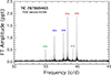 |
Fig. 2. Fourier transform of the TESS data from sectors 63–66 for TIC 28786963. The labels mark the two dipole modes (D1 and D2) and an octupole mode (O1). Each mode has two prominent components, marked a and b. The dipole components are separated by 2 νorb, and the octupole components are separated by 6 νorb. |
The echelle diagram for the pulsations of this star is shown in Figure 3. The D1 mode has a small central component, but D2 does not. The octupole mode is split by 6 νorb and has only one tiny intermediate frequency peak, which is situated at 1 νorb from the missing central frequency. There are also two low-amplitude singlet modes at 35.976 and 41.096 d−1.
 |
Fig. 3. Echelle diagram for TIC 287869463 constructed from the TESS data of sectors 63–66. This shows the frequencies of the pulsations vs. echelle phase, i.e., the frequency modulo νorb and normalized to νorb. The labeling of the components follows Fig. 2. |
The six most significant frequencies seen in the periodogram and echelle diagram, related to D1, D2, and O1, are enumerated in Table 3. These frequencies were produced from phase tracking the pulsations (see, e.g., Rowman et al. 2016, and also Appendix A) over all 12 sectors of 200 s and 600 s cadence data (where the pulsation frequencies were below the Nyquist frequency). All frequencies are referenced to a common epoch, BJD = 2 460 000. In the fifth column of Table 3, we list the mean frequency split between the two components of the particular mode. In the last column, we indicate the (orbital) period inferred from the splitting, and these values all agree to within 10−5 d of the calculated orbital period2.
Frequencies of the six prominent pulsations seen in TIC 287869463a.
The amplitudes and phases of the six pulsations as a function of TESS sector are given in the top and bottom panels of Fig. 4, respectively. The amplitudes of the two components of each of the dipoles are clearly correlated, as are the two amplitudes of the octupole mode. However, the latter are less variable than for the D1 and D2 modes. The two amplitudes for each pulsation mode are always very similar and do not vary independently.
 |
Fig. 4. Top: Variations in the dipole (red and blue) and octupole (green) component amplitudes with sector number across ∼5 yr. For each mode, the two component peaks have very similar amplitudes, and their variations are clearly tightly correlated. Bottom: Difference in phase between the two components of each of the three modes at the times of primary eclipse. To fit all three curves on the same scale, we subtracted 180 degrees from the phase difference of modes D2 and O1. Note that the phase differences remain approximately constant at either 0 or π rad. |
In the phase plot (Fig. 4, bottom panel), we show the phase difference between the two components of each mode as a function of TESS sector, all referenced to a time of primary eclipse (BJD = 2 460 014.4757). For the D1 mode, the two components are mostly in phase at the primary eclipse. The two components of the D2 and O1 modes are essentially always out of phase by 180° at the primary eclipses. (This in turn means that these modes are at an amplitude minimum at primary eclipse.) The standard errors in the phase differences are only 1.1°, 0.9°, and 3.7° for the D1, D2, and O1 modes, respectively.
We next force-fit a three-element triplet in frequency (separated by νorb) to each of the dipole modes and a seven-element septuplet to the octupole mode. We used the amplitudes and phases of the extracted mode elements to reconstruct the amplitudes of the three pulsation modes as a function of orbital phase. These results are shown in the top panel of Fig. 5. An amplitude-scaled orbital light curve is shown superposed for phasing reference. Each of the dipoles has two amplitude maxima per orbit, while the octupole has six such maxima. We find that D1 has a maximum amplitude at the eclipses, while D2 has a minimum there. The octupole mode also has a pulsation minimum at the eclipses. These all agree with the discussion above of the phase differences of the two elements of each mode (see also Fig. 4) at the time of primary eclipse. The bottom panel of Fig. 5 shows the run of reconstructed pulse phase versus orbital phase. The dipole modes have two π phase jumps each orbit, while the octupole mode has six π phase jumps.
 |
Fig. 5. Reconstructions of pulsation amplitude and phase vs. the orbital phase. The color-coding, top to bottom, is red = D1, blue = D2, and green = O1. A scaled version of the orbital light curve is superposed to guide the eye on the orbital phasing. We note the six maxima in pulsation amplitude and six π rad phase jumps per orbit for the octupole (O1). |
Several arguments indicate that the octupole mode in this star (the first such stationary ℓ = 3 sectoral mode discovered) is a single-pulsation mode split by 6 νorb, as opposed to two independent modes that are coincidentally separated by ∼6 νorb. First, the separation of the octupole mode elements corresponds to an integer multiple of the measured orbital period to one part in 105. The odds of this occurring at random for the two significant non-dipole frequencies over the pulsation range of 30–40 d−1 is only 1.7 × 10⁻⁶ (verified by Monte Carlo simulations). Second, the very similar amplitudes of the two mode components and their correlated amplitude and frequency variations over a 5-year interval (see Appendix A) also strongly suggest that these are not from independent modes. Third, a minimum or maximum at the time of the primary eclipse (minimum in this case) in this mode would occur at random only about 25% of the time3. We also note that a well-developed model (Fuller et al. 2025) predicts such modes, and this adds confidence to the interpretation that this is an octupole mode.
3. Simulations of the modes and interpretation
Our analysis of the TESS data for this star showed that we have found an octupole mode of the form
 (1)
(1)
where the Ys on the right-hand side of the top equation are ordinary spherical harmonics with ℓ = 3 and m = ±3. The additional z designation indicates that the axis of these modes lies along the rotation vector of the pulsating star, which in turn we assume is aligned with the orbital angular momentum vector (along  ). A traveling wave propagates around the stellar equator for each of these spherical harmonics. Fuller et al. (2025) showed how such modes can be coupled by perturbations on the pulsating star in a binary from tidal, Coriolis, and centrifugal forces into a stationary mode (standing wave) in the rotating stellar reference frame.
The Y33+ mode is a standing-wave sectoral octupole mode in a frame rotating with the orbital motion. Here, the plus indicates the sum, rather than the difference, between the terms on the right side of Equation (1). This mode differs from standard sectoral Y3 + 3z or Y3 − 3z modes by its stationary nature. Throughout the orbital cycle, we can therefore observe this mode from varying angles. This gives the same advantage of providing information on the geometry of the mode (and its viewing aspect) as is gained from oblique pulsation in roAp stars. Such geometric information cannot be extracted from rotationally perturbed normal sectoral octupole modes pulsating about the rotation axis.
Previously, we identified numerous stationary dipole modes formed from Y11± modes (Y1 + 1z ± Y1 − 1z) (Zhang et al. 2024; Jayaraman et al. 2024). We are also working on a smaller set of other pulsators with related quadrupole modes formed as Y22± = Y2 + 2z ± Y2 − 2z (see, e.g., Handler et al. 2025). As described in Fuller et al. (2025), there are three other perturbed stationary ℓ = 2 modes and five other ℓ = 3 modes in addition to the two described above. However, the components of these other ℓ = 3 Fuller modes are split by either two or four times the orbital frequency and can be difficult to distinguish from Y11± or Y22± modes.
In order to make some of the properties of the new stationary perturbed modes concrete, we developed a code to simulate these pulsations in a binary star system. We used two stationary spherical stars separated by the semimajor axis of the binary a. We uniformly distributed 7000 unit vectors on each star and then viewed the system from the perspective of an observer orbiting around the binary at a frequency νorb at an inclination angle i. Any pulsation mode can then be assigned to the fixed pulsating star; this mode can be either circulating or stationary4. The pulsation amplitudes were arbitrary since we have no way of calculating these a priori. At a given time, we evaluated the dot product between the viewing direction unit vector and the unit vectors over the surface of both stars. When the dot product was negative, then the observer sees that part of the star; all the visible flux (as calculated in this manner) was then summed. Eclipsed regions were also excluded from the sum. This same dot product was also used to compute the limb darkening and the projected area of the surface element. We also added a simple cosine term of 2νorb to represent an ellipsoidal light variation for aesthetic purposes.
This set of calculations was made every 120 s (to match the TESS 2-min cadence) for 50 000 steps (to roughly match three sectors of TESS data). The orbital modulations were removed from the simulated time series, as is done for the real dataset. We then took the FT of the simulated data. The entire process was then repeated for 18 orbital inclination angles between 90° and 5°. An illustrative set of simulated light curves for a Y33+ mode is shown in Fig. 6. Each light curve has six pulsational maxima per orbit with minima (in this particular case) at both eclipses. In general, the relative pulsation amplitude decreases with decreasing inclination angle and reaches zero at i = 0, as expected. We highlight the curve at i = 75° because it is close to the inclination determined for TIC 287869463 (see Sect. 4).
 |
Fig. 6. Simulated light curves of TIC 287869463 with a Y33+ pulsation mode. The orbital inclination angles in degrees are written next to the right y-axis. The orange curve for i = 75° represents the simulated light curve for the approximate inclination angle of TIC 287869463. The curves for different inclinations are shifted vertically by arbitrary amounts for clarity. |
FTs of simulated data for four different ℓ = 3 modes are shown in Fig. 7. In the upper left panel, we display the FTs for a Y33+ mode of the type detected for TIC 287869463 as a function of orbital inclination angle. There are two main peaks that are separated by 6 νorb. The smaller peaks for i ≳ 80° arise because the eclipses periodically modulate the intensity of the pulsations, a phenomenon known as spatial filtration (Gamarova et al. 2003; Reed et al. 2005; Biró & Nuspl 2011; Johnston et al. 2023; Van Reeth et al. 2023). For an inclination of ∼75° (as observed for TIC 287869463), these frequency peaks would not have been detected. In the upper right panel, we show the corresponding FTs for a Y33− mode, and the results are similar to those for a Y33+ mode. The main difference is that the small intermediate peaks are somewhat more pronounced because the pulsation amplitudes are maximum at the eclipses, rather than minimum, and this enhances the effects of the eclipses on the visibility of the pulsations. Even at i ≃ 75°, however, these smaller peaks would have been only barely detectable, however.
 |
Fig. 7. Simulated FTs for different examples of ℓ = 3 pulsation modes. The modes represented in the four panels are Y33+, Y33−, Y33x, and Y31x, clockwise starting from the upper left panel. The first two modes are defined in Sect. 3 and Equation (1). The pulsation axis of the latter two modes has been tilted into the orbital plane and lies along the tidal (or x) axis. The FT peaks are arbitrarily shifted to the left for decreasing inclination angles to avoid overlapping peaks. |
A surface plot of the Y33+ mode and the Y33− mode, as they might appear in the context of TIC 287869463, is shown in Figure 8. Note the pulsation minimum (maximum) at the time of superior conjunction in the Y33+ (Y33−) mode.
 |
Fig. 8. Diagrams showing the flux perturbation across the surface of a star pulsating in the Y33+ mode (top) and Y33− mode (bottom). The diagram corresponds to orbital phase zero for an observer viewing at at inclination i = 55° relative to the orbital axis. The observed phase of the amplitude modulation of the O1 mode is consistent with that of a Y33+ mode. |
In the lower two panels of Fig. 7, we show the FTs for simulated data of two different ℓ = 3 modes, namely a Y33x and Y31x mode. Here, the x signifies that the pulsation axis is tilted into the orbital plane and lies along the tidal axis. As mentioned above, these are tidally tilted pulsations, and traveling waves propagate around the x-axis. As shown by the simulations, there are numerous intermediate peaks out to ±3 νorb. We recall that the central peak of each multiplet is the only pulsation mode frequency; all of the other components of the multiplet are Fourier descriptions of the observed pulsation amplitude and phase modulating with changing orbital aspect. These multiplets in the lower two panels are very different from what is observed in TIC 287869463. We simulated all combinations of traveling and stationary modes around all three axes x, y, and z with ℓ = 3, and the only mode that fits the observational data (FT and the phasing of amplitudes and pulse phases with respect to the eclipses) for TIC 287869463 is a Y33+ octupole Fuller mode.
4. Analysis of the binary system
To evaluate the properties of the two stars in TIC 287869463, we simultaneously fit the spectral energy distribution (SED) curve and the TESS light curve. We employed a Markov chain Monte Carlo (MCMC) algorithm to fit for the stellar masses M1 and M2 (where M1 is the more massive pulsating star), the system age, the orbital inclination angle i, interstellar extinction, AV, and the distance. The latter two parameters were fixed at the values from Gaia. In total, there were between four and six free parameters. We assumed that the binary had evolved in a coeval fashion, that is, no prior mass transfer or mass loss from the system. We were thus able to use stellar evolution models (Choi et al. 2016; Dotter 2016) to determine the radii and Teff of both stars, which are uniquely determined given their masses and age.
We collected the available archival spectral flux measurements (SED points) from 0.15 to 11.6 μm. These data were accessed from VizieR5 (Ochsenbein et al. 2000), which in turn uses the systematic sky coverage of such surveys as Panoramic Survey Telescope and Rapid Response System (Pan-STARRS; Chambers et al. 2016), Sloan Digital Sky Survey (SDSS; Gunn et al. 1998), Two Micron All Sky Survey (2MASS; Skrutskie et al. 2006), Wide-field Infrared Survey Explorer (WISE; Cutri et al. 2013), Galaxy Evolution Explorer (GALEX; Bianchi et al. 2017), and Global Astrometric Interferometer for Astrophysics (Gaia; Gaia Collaboration 2021). More details about this type of SED fitting for binary star systems are given in Jayaraman et al. (2024), Handler et al. (2025), Yakut et al. (2025a,b).
The input information we used included (i) 23 available SED points spanning 0.15 μm to 11.6 μm, (ii) an approximate value for K1 of the radial velocity (RV) curve6, (iii) the eclipsing light-curve profile, (iv) the Gaia distance of 1086 ± 3 pc (Bailer-Jones et al. 2021), and a Gaia value for AG of 0.7097. Additionally, we used the MESA Isochrones and Stellar Tracks (MIST) evolution tracks (Paxton et al. 2011, 2015; Choi et al. 2016; Dotter 2016; Paxton 2019) to relate the stellar mass and age to its radius and Teff. In order to compute the model stellar spectra from the radii and Teff of the stars, we used the Castelli & Kurucz model stellar atmospheres (Castelli & Kurucz 2003), assuming solar metallicity. Finally, we corrected for interstellar extinction using the prescription presented in Cardelli et al. (1989).
When a composite SED of two or more stars is fit, it is important to have additional constraints among the properties of one star and the other(s). In particular, the eclipsing light curve in this system provides important information about parameters such as Teff, 2/Teff, 1, R2/R1, R1/a, and the orbital inclination angle, where a is the semimajor axis of the system. Since well-developed light-curve emulators such as PHysics Of Eclipsing BinariEs (PHOEBE; Prša & Zwitter 2005) are not designed to work jointly with SED fitting codes, we incorporated our own simple light-curve emulator to help the SED fitter separate the light contribution from the two stars more properly (Jayaraman et al. 2024). This light-curve emulator uses two spherical stars with limb darkening to generate eclipses. The out-of-eclipse behavior is described by three sinusoids of the form cos(ωorbt), cos(2ωorbt), and sin(ωorbt) to represent effects such as ellipsoidal light variations, illumination effects, Doppler boosting, and corotating spots on the cooler star (see, e.g., Kopal 1959; Carter et al. 2011).
The best-fitting SED and light-curve models are shown in the top and bottom panels of Fig. 9. The best-fitting system parameters derived from these fits are summarized in Table 4. The luminosity of the primary star, with a mass of 2.2 M⊙, radius 2.6 R⊙, and Teff, 1 = 8734 K, is typical of a δ Scuti star, with Teff near the blue border of the δ Sct instability strip. The pulsator parameters place it between the Balona et al. (2015)δ Scuti-category boxes 4 and 7 in their Fig. 2. The pulsations of pulsators in these categories can reach ∼50 d−1, and there are many such systems with pulsations in a range similar to what we see in TIC 287869463.
 |
Fig. 9. Top panel: Spectral energy distribution fit for TIC 287869463. The blue curve shows the model spectrum for the primary star (the pulsator), and the red curve represents the model spectrum for the cooler smaller secondary star. The black curve that nearly coincides with the red curve is the sum of the model fluxes. The orange points are measured SED points from the literature (for the SED fitting techniques and the origin of the data points, see Sect. 4). Bottom panel: Light-curve fit using our custom light-curve emulator. The black curve shows the Fourier-reconstructed light curve (i.e., the data), and the red curve shows the model fit (see text for details). |
Binary system parametersa.
Finally, we point out that even though the secondary star contributes less than 1% of the system luminosity, we can be confident that we measured its parameters because there are numerous constraints between the secondary and the primary other than from the SED, for instance, K1, R2/R1, and T2/T1. Therefore, the primary star largely accounts for matching the SED, while the properties of the secondary star (including its contribution to the SED) come from the relative relations listed above, and from a common age.
5. Discussion
While carrying out a large-scale search for Fuller-mode pulsators in TESS data, we discovered an unprecedented octupole mode in a δ Scuti star. The mode is characterized by two peaks in the Fourier transform separated by 6 νorb. This splitting corresponds to six times the orbital frequency to within an accuracy of one part in 105. We argue that this cannot be just two random and unrelated modes of the pulsating star, but must comprise a single mode.
This octupole mode is actually a combination of ordinary Y3 + 3 and Y3 − 3 modes that are aligned with the stellar rotation axis. These are combined into a new eigenmode of the star by binary perturbations, and we call it a Fuller Y33+ mode (Fuller et al. 2025). We presented a number of compelling reasons why the octupole mode cannot plausibly be two independent modes whose frequencies are accidentally aligned in the echelle diagram. This is the first securely identified octupole mode in any δ Scuti star, and the first Fuller-type ℓ = 3 stationary sectoral mode found in any star, including the Sun.
As we show in the appendix, the pulsation frequencies of the dipole and octupole modes were found to steadily increase with time, all at different rates. However, the splits in the mode frequencies remain constant at an integer multiple of the orbital frequency.
Because of geometric cancellation of higher-order ℓ modes over the visible hemisphere of pulsating stars, the visibility of a pulsation mode decreases sharply with increasing ℓ. To investigate the visibility of higher-degree modes, we followed the approach described in Daszyńska-Daszkiewicz et al. (2002). As a first step, we approximated the mode visibility by the disk-averaging factor
 (2)
(2)
where μ is the cosine of the angle between the observer line of sight and the local surface normal, and h is the limb-darkening function. This should be reasonably accurate when the effects of rapid rotation and tidal interaction are neglected. In a more general approach, as in the case of the star we studied, the mode visibility may also depend on the azimuthal order m.
We show a plot of the visibility of pulsation modes in a star like TIC 287869463 in Fig. 10 as a function of ℓ for four different filters, including a red filter, which is a reasonable approximation to the TESS bandpass (the results are also given numerically in Table 5). Dipole and quadrupole modes (ℓ = 1 and ℓ = 2, respectively) have relatively high visibilities of 0.7 and 0.3, respectively. However, for octupole modes (ℓ = 3), the visibility drops abruptly to 0.037 (for the red filter). In TIC 287869463, the dipole mode amplitudes are 1.8 mmag and 0.8 mmag. However, the amplitude of the octupole mode at 0.4 mmag is not too far below this. When we renormalized this according to the relative visibilities, the intrinsic amplitude of the octupole mode was found to be ∼10 mmag. Pulsation amplitudes of this size are fairly common among δ Scuti stars.
 |
Fig. 10. Mode visibility diagram as a function of ℓ. These visibilities were calculated as in Daszyńska-Daszkiewicz et al. (2002) for the BVRI passbands; the red passband matches that of TESS best. |
Mode visibilitiesa.
This exercise also showed that even hexadecapole modes with ℓ = 4 are expected to be as straightforward to detect as the octupole mode found here. However, higher modes with ℓ ≥ 5 will be very difficult to detect.
It is also worth noting that according to the simulations of Daszyńska-Daszkiewicz et al. (2006), the octupole mode should be relatively easy to identify from radial-velocity variations. Therefore, time-series spectroscopy might be used to validate our identification of the octupole mode for TIC 287869463.
Finally, we show model evolution tracks in the HR diagram for several sets of model parameters in Figure 11, along with a comparison to the stellar values we derived for the TIC 287869463 pulsator. The evolutionary models were computed with the Warsaw-New Jersey code (e.g., Pamyatnykh 1999) adopting the OPAL opacity tables (Iglesias & Rogers 1996) and the chemical mixture of Asplund et al. (2009). With the accurately determined stellar parameters, including the mass and radius, we expect strong constraints from seismic modeling of this star, for example, on the metallicity Z, the efficiency of outer-layer convection αMLT, and the overshooting distance αov. This will be the subject of our follow-up studies of this object.
 |
Fig. 11. Six different evolution tracks in the HR diagram compared to the measured luminosity and Teff of TIC 287869463. The parameters that are varied in the different tracks involve metallicity Z, αMLT, mass, rotation velocity, and convective overshooting, αov (see text for details). |
Acknowledgments
RJ is currently supported by a Klarman Fellowship from the College of Arts & Sciences at Cornell University. This project has received partial funding from the HUN-REN Hungarian Research Network. T.B. acknowledges the financial support of the Hungarian National Research, Development and Innovation Office – NKFIH Grant OTKA K-147131. VBK is grateful for financial support from NASA grant 80NSSC22K0747. GH thanks the Polish National Center for Science (NCN) for support through grant 2021/43/B/ST9/02972. JDD thanks the Polish National Center for Science (NCN) for support through grant 2023/50/A/ST9/00144. This paper includes data collected by the TESS mission. Funding for the TESS mission is provided by the NASA Science Mission Directorate. The QLP data used in this work were obtained from MAST (Huang 2020), hosted by the Space Telescope Science Institute (STScI). STScI is operated by the Association of Universities for Research in Astronomy, Inc., under NASA contract NAS 5-26555. This work also presents results from the European Space Agency (ESA) space mission Gaia. Gaia data are being processed by the Gaia Data Processing and Analysis Consortium (DPAC). Funding for the DPAC is provided by national institutions, in particular the institutions participating in the Gaia Multilateral Agreement. The Gaia mission website is https://www.cosmos.esa.int/web/gaia. The Gaia archive website is https://gea.esac.esa.int/archive/. Some of the SED fluxes and magnitudes were obtained with the Wide-field Infrared Survey Explorer, which is a joint project of the University of California, Los Angeles, and the Jet Propulsion Laboratory/California Institute of Technology, funded by the National Aeronautics and Space Administration. Additionally, some of the SED fluxes and magnitudes were obtained with the Two Micron All Sky Survey, which is a joint project of the University of Massachusetts and the Infrared Processing and Analysis Center/California Institute of Technology, funded by the National Aeronautics and Space Administration and the National Science Foundation. We used the Simbad service operated by the Centre des Donnés Stellaires (Strasbourg, France). This research has also made use of the VizieR catalogue access tool, CDS, Strasbourg, France (DOI : 10.26093/cds/vizier). The original description of the VizieR service was published in Ochsenbein et al. (2000).
References
- Aerts, C., De Cat, P., Cuypers, J., et al. 1998, A&A, 329, 137 [NASA ADS] [Google Scholar]
- Aerts, C., Christensen-Dalsgaard, J., & Kurtz, D. W. 2010, Asteroseismology (Springer) [Google Scholar]
- Asplund, M., Grevesse, N., Sauval, A. J., & Scott, P. 2009, ARA&A, 47, 481 [NASA ADS] [CrossRef] [Google Scholar]
- Astropy Collaboration (Robitaille, T. P., et al.) 2013, A&A, 558, A33 [NASA ADS] [CrossRef] [EDP Sciences] [Google Scholar]
- Astropy Collaboration (Price-Whelan, A. M., et al.) 2018, AJ, 156, 123 [Google Scholar]
- Astropy Collaboration (Price-Whelan, A. M., et al.) 2022, ApJ, 935, 167 [NASA ADS] [CrossRef] [Google Scholar]
- Bailer-Jones, C. A. L., Rybizki, J., Fouesneau, M., Demleitner, M., & Andrae, R. 2021, AJ, 161, 147 [Google Scholar]
- Balona, L. A., Daszyńska-Daszkiewicz, J., & Pamyatnykh, A. A. 2015, MNRAS, 452, 3073 [Google Scholar]
- Bianchi, L., Shiao, B., & Thilker, D. 2017, ApJS, 230, 24 [Google Scholar]
- Biró, I. B., & Nuspl, J. 2011, MNRAS, 416, 1601 [CrossRef] [Google Scholar]
- Cardelli, J. A., Clayton, G. C., & Mathis, J. S. 1989, ApJ, 345, 245 [Google Scholar]
- Carter, J., Rappaport, S., & Fabrycky, D. 2011, ApJ, 728, 139 [NASA ADS] [CrossRef] [Google Scholar]
- Castelli, F., & Kurucz, R. L. 2003, IAU Symp., 210, A20 [Google Scholar]
- Çelik, E., & Kahraman Aliçavuş, F. 2024, PASJ, 76, 787 [Google Scholar]
- Chambers, K. C., Magnier, E. A., Metcalfe, N., et al. 2016, ArXiv e-prints [arXiv:1612.05560] [Google Scholar]
- Choi, J., Dotter, A., Conroy, C., et al. 2016, ApJ, 823, 102 [Google Scholar]
- Cotton, D. V., Buzasi, D. L., Aerts, C., et al. 2022, NatAs, 6, 154 [Google Scholar]
- Cowling, T. G. 1941, MNRAS, 101, 367 [NASA ADS] [Google Scholar]
- Cutri, R. M., Wright, E. L., Conrow, T., et al. 2013, Explanatory Supplement to the AllWISE Data Release Products [Google Scholar]
- Danielski, C., Babusiaux, C., Ruiz-Dern, L., Sartoretti, P., & Arenou, F. 2018, A&A, 614, A19 [NASA ADS] [CrossRef] [EDP Sciences] [Google Scholar]
- Daszyńska-Daszkiewicz, J., Dziembowski, W. A., Pamyatnykh, A. A., & Goupil, M.-J. 2002, A&A, 392, 151 [NASA ADS] [CrossRef] [EDP Sciences] [Google Scholar]
- Daszyńska-Daszkiewicz, J., Dziembowski, W. A., & Pamyatnykh, A. A. 2006, A&A, 77, 113 [Google Scholar]
- Di Mauro, M. P., Cardini, D., Catanzaro, G., et al. 2011, MNRAS, 415, 3783 [NASA ADS] [CrossRef] [Google Scholar]
- Dotter, A. 2016, ApJS, 222, 8 [Google Scholar]
- Dziembowski, W. A. 1977, Acta Astr., 27, 203 [Google Scholar]
- Eddington, A. S. 1919a, MNRAS, 79, 171 [NASA ADS] [CrossRef] [Google Scholar]
- Eddington, A. S. 1919b, MNRAS, 79, 177 [NASA ADS] [Google Scholar]
- Eddington, A. S. 1926, The Internal Constitution of the Stars (Cambridge: Cambridge University Press) [Google Scholar]
- Feinstein, A. D., Montet, B. T., Foreman-Mackey, D., et al. 2019, PASP, 131, 94502 [Google Scholar]
- Fuller, J., Kurtz, D., Handler, G., & Rappaport, S. 2020, MNRAS, 498, 5730 [NASA ADS] [CrossRef] [Google Scholar]
- Fuller, J., Rappaport, S., Jayaraman, R., Kurtz, D., & Handler, G. 2025, ApJ, 979, 80 [Google Scholar]
- Gaia Collaboration (Brown, A. G. A., et al.) 2021, A&A, 649, A1 [NASA ADS] [CrossRef] [EDP Sciences] [Google Scholar]
- Gamarova, A. Yu., Mkrtichian, D. E., Rodriguez, E., Costa, V., & Lopez-Gonzalez, M. J. 2003, ASPC, 292, 369 [Google Scholar]
- Gunn, J. E., Carr, M., Rockosi, C., et al. 1998, AJ, 116, 3040 [NASA ADS] [CrossRef] [Google Scholar]
- Handler, G., Kurtz, D. W., Rappaport, S. A., et al. 2020, NatAs, 4, 684 [Google Scholar]
- Handler, G., Rappaport, S., Jones, D., et al. 2025, A&A, 702, A104 [NASA ADS] [CrossRef] [EDP Sciences] [Google Scholar]
- Harris, C. R., Millman, K. J., van der Walt, S. J., et al. 2020, Nature, 585, 357 [NASA ADS] [CrossRef] [Google Scholar]
- Huang, C. X. 2020, TESS Lightcurves From The MIT Quick-Look Pipeline ("QLP"), STScI/MAST [Google Scholar]
- Hunter, J. D. 2007, CSE, 9, 90 [Google Scholar]
- Iglesias, C. A., & Rogers, F. J. 1996, ApJ, 464, 943 [NASA ADS] [CrossRef] [Google Scholar]
- Jayaraman, R., Handler, G., Rappaport, S., et al. 2022, ApJ, 928, L14 [NASA ADS] [CrossRef] [Google Scholar]
- Jayaraman, R., Rappaport, S., Powell, B., et al. 2024, ApJ, 975, 121 [Google Scholar]
- Johnston, C., Tkachenko, A., Van Reeth, T., et al. 2023, A&A, 670, A167 [NASA ADS] [CrossRef] [EDP Sciences] [Google Scholar]
- Katz, D., Sartoretti, P., Guerrier, A., et al. 2023, A&A, 674, A5 [NASA ADS] [CrossRef] [EDP Sciences] [Google Scholar]
- Kjeldsen, H., Bedding, T. R., Butler, R. P., et al. 2005, ApJ, 635, 1281 [NASA ADS] [CrossRef] [Google Scholar]
- Kopal, Z. 1959, Close Binary Systems (London: Chapman& Hall), Int. Astrophys. Ser. [Google Scholar]
- Kostov, V., Powell, B. P., Fornear, A. U., et al. 2025, ApJS, 279, 50 [Google Scholar]
- Kovács, G., Zucker, S., & Mazeh, T. 2002, A&A, 391, 369 [Google Scholar]
- Kunimoto, M., Huang, C., Tey, E., et al. 2021, Res. Notes AAS, 5, 234 [Google Scholar]
- Kunimoto, M., Tey, E., Fong, W., et al. 2022, Res. Notes AAS, 6, 236 [Google Scholar]
- Kurtz, D. W. 1982, MNRAS, 200, 807 [NASA ADS] [CrossRef] [Google Scholar]
- Kurtz, D. W. 2022, ARA&A, 60, 31 [NASA ADS] [CrossRef] [Google Scholar]
- Kurtz, D. W., Handler, G., Rappaport, S., et al. 2020, MNRAS, 494, 5118 [Google Scholar]
- Larson, T., & Schou, J. 2011, JPhCS, 271, 12062 [Google Scholar]
- Larson, T. P., & Schou, J. 2015, Sol. Phys., 290, 3221 [NASA ADS] [CrossRef] [Google Scholar]
- Lee, J. W., Hong, K., Park, J.-H., Wolf, M., & Kim, D.-J. 2023, AJ, 165, 159 [Google Scholar]
- Lehmann, H., Dervişoǧlu, A., Mkrtichian, D. E., et al. 2020, A&A, 644, A121 [NASA ADS] [CrossRef] [EDP Sciences] [Google Scholar]
- Lenz, P., & Breger, M. 2005, CoAst, 146, 53 [NASA ADS] [Google Scholar]
- Lightkurve Collaboration (Cardoso, J. V. d. M., et al.) 2018, Astrophysics Source Code Library [record ascl:1812.013] [Google Scholar]
- Mowlavi, N., Holl, B., Lecoeur-Taïbi, I., et al. 2023, A&A, 674, A16 [NASA ADS] [CrossRef] [EDP Sciences] [Google Scholar]
- Ochsenbein, F., Bauer, P., & Marcout, J. 2000, A&AS, 143, 23 [NASA ADS] [CrossRef] [EDP Sciences] [Google Scholar]
- O’Connell, D. J. K. 1951, Publ. Riverview Coll. Obs., 2, 85 [Google Scholar]
- Pamyatnykh, A. A. 1999, Acta Astron., 49, 119 [Google Scholar]
- Paxton, B. 2019, ApJS, 243, 10 [NASA ADS] [CrossRef] [Google Scholar]
- Paxton, B., Bildsten, L., Dotter, A., et al. 2011, ApJS, 192, 3 [Google Scholar]
- Paxton, B., Marchant, P., Schwab, J., et al. 2015, ApJS, 220, 15 [Google Scholar]
- Powell, B., Kostov, V., Rappaport, S., et al. 2021, AJ, 161, 162 [NASA ADS] [CrossRef] [Google Scholar]
- Prša, A., & Zwitter, T. 2005, ApJ, 628, 426 [Google Scholar]
- Rappaport, S., Kurtz, D. W., Handler, G., et al. 2021, MNRAS, 503, 254 [NASA ADS] [Google Scholar]
- Rappaport, S., Borkovits, T., Gagliano, R., et al. 2022, MNRAS, 513, 434 [Google Scholar]
- Reed, M. D., Brondel, B. J., & Kawaler, S. D. 2005, ApJ, 634, 602 [NASA ADS] [CrossRef] [Google Scholar]
- Ricker, G. R., Winn, J. N., Vanderspek, R., et al. 2015, JATIS, 1, 14003 [Google Scholar]
- Rowman, D. M., Kurtz, D. W., Breger, M., Murphy, S., & Holdsworth, D. L. 2016, MNRAS, 460, 1970 [NASA ADS] [CrossRef] [Google Scholar]
- Scherrer, P. H., Schou, J., Bush, R. I., et al. 2012, SoPh, 275, 207 [Google Scholar]
- Shibahashi, H., & Kurtz, D. W. 2012, MNRAS, 422, 738 [Google Scholar]
- Skrutskie, M. F., Cutri, R. M., Stiening, R., et al. 2006, AJ, 131, 1163 [NASA ADS] [CrossRef] [Google Scholar]
- Stassun, K. G., Oelkers, R. J., Paegert, M., et al. 2019, AJ, 158, 138 [Google Scholar]
- Stello, D., Cantiello, M., Fuller, J., et al. 2016, Nature, 529, 364 [Google Scholar]
- Van Reeth, T., Johnston, C., Southworth, J., et al. 2023, A&A, 671, A121 [NASA ADS] [CrossRef] [EDP Sciences] [Google Scholar]
- Virtanen, P., Gommers, R., Oliphant, T. E., et al. 2020, NatMe, 17, 261 [NASA ADS] [Google Scholar]
- Yakut, K., Kalomeni, B., & Rappaport, S. 2025a, MNRAS, 542, 1817 [Google Scholar]
- Yakut, K., Kalomeni, B., Rappaport, S., & Kostov, V. 2025b, MNRAS, 544, 271 [Google Scholar]
- Yuan, J.-Zh., & Qian, Sh.-B. 2019, Res. A&Ap, 19, 128 [Google Scholar]
- Zhang, V., Rappaport, S., Jayaraman, R., et al. 2024, MNRAS, 528, 3378 [Google Scholar]
We take the  and
and  directions to lie along the angular momentum vector of the binary and the direction in the orbital plane perpendicular to the tidal axis, respectively.
The apparent orbital period also changes with time, and the cited orbital period is also referenced to this same epoch of BJD = 2 460 000 (see Appendix A).
Because in such an octupole mode, there will be either a minimum or maximum every 30°, and we have an accurate determination of the mode phase to within ±3.7°.
We assumed that the fractional flux, δF/F, emerging from each surface element of the star due to the pulsation is simply proportional to the Yℓ, m of the particular mode being simulated.
We used the Gaia parameter RV_amp_robust of 144 km s−1 as a proxy for twice the RV amplitude K1 (e.g., Katz et al. 2023).
This translates into an AV of ∼0.84 using either the rule-of-thumb factor of 1.2 or the detailed expression of Danielski et al. (2018); in particular their Equation (3) and coefficients from row 5 of their Table 2.
Appendix A: Changes in the pulsation frequencies and the orbital period
The pulsation frequencies and the orbital period appear to be nearly constant across the 200-s cadence data from the four contiguous TESS sectors 63-66, or even to some extent when we include the final three sectors of 200-s cadence—separated from the former sectors by about 700 d. However, the apparently constant pulsation frequencies are seen to be clearly varying once we add five earlier sectors with 600-s cadence data (sectors between S30 and S39). Overall, after analyzing the available TESS data between sectors S30 and S93, the pulsation frequencies are all found to be significantly increasing with time. The orbital frequency can be tracked to even earlier times by using six sectors between S3 and S13 with 30-min cadence, and νorb is also found to be increasing with time. We thus sought to characterize the frequency changes in the pulsations as well as in the orbit.
To track the pulsation phases ϕ (see also Rowman et al. 2016), we fit a sine curve of the form Acos[ω(t−tecl)−ϕ] to represent a pulsation over an interval of, say, half of a full TESS sector (∼12 d). We needed to consider sufficiently long intervals because some of the pulsation peaks are within a fraction of 1 d−1 of other peaks. The reference time, tecl is the time of a primary eclipse, e.g., BJD 2460014.476. We then fit for A and ϕ and stepped the fitting window forward in time by a fraction of a TESS sector.
The results of tracking the phase for each of the 6 pulsation frequencies are given in Figure A.1. Each panel displays the equivalent Eclipse Timing Variation (ETV) curve for both components of a given pulsation mode: D1a and D1b, D2a and D2b (top two panels) and O1a and O1b in the lower left panel. Note that for mode D1, the a and b components track each other very well, and we saw in Fig. 4 that indeed these two components are always in phase at the primary eclipses. By contrast, we can see from the ETVs of D2 and O1 that the ETV curves for the two components are separated by close to half a pulsation period, consistent with the fact that the two components of both modes remain out of phase at the primary eclipses over all the sectors with 10-min or better cadence.
 |
Fig. A.1. ETV curves for each component of the three pulsation modes, D1, D2, and O1, as well as from the binary orbital period. All four curves show decreasing periods with time, but not at the same rates. All phases are referenced to the times of a primary eclipse, i.e., at BJD - 2,456,014.4757. Note that the vertical scale for the D1 ETVs is exactly 1/3 that for the D2 and O1 ETVs. In turn, the vertical scale for the orbital ETV curve is 4/5 that of the D1 ETVs. |
The final panel in Fig. A.1 shows the ETV curve for the orbital period. This shows that Porb is also apparently decreasing with time. If we interpret this as an orbital decay, then the decay timescale of just ∼2 × 10⁵ yr seems rather implausible. Alternatively, we might interpret the curve as a portion of a Doppler delay orbit caused by an orbiting third body. Unfortunately, the duration of available TESS data is insufficient to determine an outer orbit for a putative third body. However, for one of the shorter allowed orbits of 15 yr, the semimajor axis is 950 light-seconds (for an assumed circular orbit), and the corresponding mass function is f(M)≃0.03 M⊙. For a binary mass of 3 M⊙ (see Table 4), this yields a value of M3sin3i of about 0.75 M⊙. A third body of such a mass would not have contributed sufficient light to the SED to have been unequivocally detected, especially for outer inclination angles of ≳75°. We note that the known secondary in the binary contributes only ≲0.01 of the system luminosity, and a comparable third star would barely perturb the SED.
Returning to the systematic nonlinear behavior in the ETV curves for the pulsations, we examine what the consequences would be for different assumptions about the nature of the nonlinear ETV curve observed for the orbit. Suppose that a Fuller mode pulsation frequency is νp, and that it is physically changing with time as  . The splitting with the orbit will be ±m νorb (see, e.g., Shibahashi & Kurtz 2012). Now, we also allow that the orbital frequency is physically changing as
  . This means that the two components of the mode (upper and lower) should follow different functions of time:
 (A.1)
(A.1)
 (A.2)
(A.2)
In turn, if we were to measure the  of the upper and lower components, we should find
 (A.3)
(A.3)
 (A.4)
(A.4)
with a difference in  of
of  . From Table A.1 we can see that the differences between the
  terms of the upper and lower frequency components are not statistically significant, and the uncertainties are ∼10−7 d−2. For the octupole mode, we might expect a change in the difference of the
  s by about 6 × 9 × 10−9 = 5.4 × 10⁻⁸ d−2 due to the changing orbit. This is smaller than the uncertainty in the difference in
  listed in Table A.1 for the octupole mode. Thus, we cannot quite use this effect to test for a decaying orbit.
Summary of frequencies and frequency derivatives in TIC 287869463a
For Doppler shifts of the binary (which include the pulsating star) the quantity  would be constant. So, we should find that all the pulsation components have
  , or
, or  d−2. In all cases, this is less than the values of
  for the pulsations listed in Table A.1, but would be readily detectable if we could separate the Doppler from other natural changes in pulse frequency.
Regarding the observed (or apparent) changes in the orbital ETV curve, we point out that many such close binaries containing an early-type star exhibit ETVs that have nonlinear variations on long timescales (decades or even centuries) that are almost certainly neither actual orbital period changes (i.e., orbital decay) nor third-body induced light travel-time effects. Some examples of very irregular and unexplained ETVs are the cases of XZ And (Yuan & Qian 2019), X Tri (Lee et al. 2023), RZ Cas (Lehmann et al. 2020), and Y Cam (Çelik & Kahraman Aliçavuş 2024). While we are confident in the nonlinear behavior of the TIC 287869463 orbital ETV curve, we cannot be certain what causes this behavior. Therefore, at least tentatively, we take all the  s for the pulsations to be independent of the orbit, and for the orbital
  to be due to neither an orbital decay nor an orbital Doppler shift.
All Tables
All Figures
|
Fig. 1. Light curves for TIC 287869463. Top: 5-d segment of the raw TESS light curve. The pulsations superposed on the eclipsing light curve are readily apparent. Bottom: Fourier-reconstructed light curve from the first 60 orbital harmonics. We used only the cosine terms in the reconstruction to remove a small time-varying O’Connell effect (O’Connell 1951), presumably arising from star spots on the cooler companion star. |
| In the text | |
|
Fig. 2. Fourier transform of the TESS data from sectors 63–66 for TIC 28786963. The labels mark the two dipole modes (D1 and D2) and an octupole mode (O1). Each mode has two prominent components, marked a and b. The dipole components are separated by 2 νorb, and the octupole components are separated by 6 νorb. |
| In the text | |
|
Fig. 3. Echelle diagram for TIC 287869463 constructed from the TESS data of sectors 63–66. This shows the frequencies of the pulsations vs. echelle phase, i.e., the frequency modulo νorb and normalized to νorb. The labeling of the components follows Fig. 2. |
| In the text | |
|
Fig. 4. Top: Variations in the dipole (red and blue) and octupole (green) component amplitudes with sector number across ∼5 yr. For each mode, the two component peaks have very similar amplitudes, and their variations are clearly tightly correlated. Bottom: Difference in phase between the two components of each of the three modes at the times of primary eclipse. To fit all three curves on the same scale, we subtracted 180 degrees from the phase difference of modes D2 and O1. Note that the phase differences remain approximately constant at either 0 or π rad. |
| In the text | |
|
Fig. 5. Reconstructions of pulsation amplitude and phase vs. the orbital phase. The color-coding, top to bottom, is red = D1, blue = D2, and green = O1. A scaled version of the orbital light curve is superposed to guide the eye on the orbital phasing. We note the six maxima in pulsation amplitude and six π rad phase jumps per orbit for the octupole (O1). |
| In the text | |
|
Fig. 6. Simulated light curves of TIC 287869463 with a Y33+ pulsation mode. The orbital inclination angles in degrees are written next to the right y-axis. The orange curve for i = 75° represents the simulated light curve for the approximate inclination angle of TIC 287869463. The curves for different inclinations are shifted vertically by arbitrary amounts for clarity. |
| In the text | |
|
Fig. 7. Simulated FTs for different examples of ℓ = 3 pulsation modes. The modes represented in the four panels are Y33+, Y33−, Y33x, and Y31x, clockwise starting from the upper left panel. The first two modes are defined in Sect. 3 and Equation (1). The pulsation axis of the latter two modes has been tilted into the orbital plane and lies along the tidal (or x) axis. The FT peaks are arbitrarily shifted to the left for decreasing inclination angles to avoid overlapping peaks. |
| In the text | |
|
Fig. 8. Diagrams showing the flux perturbation across the surface of a star pulsating in the Y33+ mode (top) and Y33− mode (bottom). The diagram corresponds to orbital phase zero for an observer viewing at at inclination i = 55° relative to the orbital axis. The observed phase of the amplitude modulation of the O1 mode is consistent with that of a Y33+ mode. |
| In the text | |
|
Fig. 9. Top panel: Spectral energy distribution fit for TIC 287869463. The blue curve shows the model spectrum for the primary star (the pulsator), and the red curve represents the model spectrum for the cooler smaller secondary star. The black curve that nearly coincides with the red curve is the sum of the model fluxes. The orange points are measured SED points from the literature (for the SED fitting techniques and the origin of the data points, see Sect. 4). Bottom panel: Light-curve fit using our custom light-curve emulator. The black curve shows the Fourier-reconstructed light curve (i.e., the data), and the red curve shows the model fit (see text for details). |
| In the text | |
|
Fig. 10. Mode visibility diagram as a function of ℓ. These visibilities were calculated as in Daszyńska-Daszkiewicz et al. (2002) for the BVRI passbands; the red passband matches that of TESS best. |
| In the text | |
|
Fig. 11. Six different evolution tracks in the HR diagram compared to the measured luminosity and Teff of TIC 287869463. The parameters that are varied in the different tracks involve metallicity Z, αMLT, mass, rotation velocity, and convective overshooting, αov (see text for details). |
| In the text | |
|
Fig. A.1. ETV curves for each component of the three pulsation modes, D1, D2, and O1, as well as from the binary orbital period. All four curves show decreasing periods with time, but not at the same rates. All phases are referenced to the times of a primary eclipse, i.e., at BJD - 2,456,014.4757. Note that the vertical scale for the D1 ETVs is exactly 1/3 that for the D2 and O1 ETVs. In turn, the vertical scale for the orbital ETV curve is 4/5 that of the D1 ETVs. |
| In the text | |
Current usage metrics show cumulative count of Article Views (full-text article views including HTML views, PDF and ePub downloads, according to the available data) and Abstracts Views on Vision4Press platform.
Data correspond to usage on the plateform after 2015. The current usage metrics is available 48-96 hours after online publication and is updated daily on week days.
Initial download of the metrics may take a while.