


| Issue |
A&A
Volume 710, June 2026
|
|
|---|---|---|
| Article Number | A273 | |
| Number of page(s) | 9 | |
| Section | Catalogs and data | |
| DOI | https://doi.org/10.1051/0004-6361/202659220 | |
| Published online | 18 June 2026 | |
Mapping X-ray conditions in the habitable zones of exoplanet host stars with SRG/eROSITA
1
Max-Planck-Institut für extraterrestrische Physik,
Gießenbachstraße 1,
85748
Garching,
Germany
2
NASA Goddard Space Flight Center,
Greenbelt,
MD
20771,
USA
3
Institut für Astronomie & Astrophysik, Eberhard Karls Universität Tübingen,
Sand 1,
72076
Tübingen,
Germany
★ Corresponding author: This email address is being protected from spambots. You need JavaScript enabled to view it.
Received:
30
January
2026
Accepted:
21
May
2026
Abstract
Stellar high-energy radiation is a key driver of atmospheric erosion and evolution in exoplanets, directly affecting their long-term habitability. We present a comprehensive study on stellar high-energy radiation and its impact on exoplanetary atmospheres, leveraging data from the eROSITA telescope array aboard the Spektrum Rötgen Gamma (SRG) satellite. Our sample consists of 3750 main-sequence stars identified via cross-matching with Gaia DR3. Utilizing X-ray spectral fits from the eROSITA catalog, we computed X-ray luminosities (LX) and extreme-ultraviolet (EUV) luminosities (LEUV), derived from scaling relationships, which we used to derive the soft X-ray flux, i.e., combined X-ray and EUV (XUV) fluxes, at the habitable zone (FXUV,HZ). We find that the majority of stars in our sample are significantly more XUV-active than the Sun, with habitable zone fluxes ranging from 10° to 10° erg cm−2 s−1. The ratio LXUV/Lbol is found to be higher for cooler, magnetically active stars, highlighting their potentially hazardous nature for planetary atmospheres. Applying the energy-limited escape model, we computed atmospheric mass-loss rates for hypothetical Earth-like planets located at the habitable zone of each star. We also present local maps for distances up to 500 pc of the average XUV flux, revealing “hazard zones” where stellar radiation could significantly influence planetary atmospheric evolution. This work demonstrates the power of X-ray surveys in constraining the high-energy environments of exoplanets and underscores the critical role of stellar activity in planetary habitability.
Key words: planets and satellites: atmospheres / planet-star interactions / X-rays: stars
© The Authors 2026
 Open Access article, published by EDP Sciences, under the terms of the Creative Commons Attribution License (https://creativecommons.org/licenses/by/4.0), which permits unrestricted use, distribution, and reproduction in any medium, provided the original work is properly cited.
This article is published in open access under the Subscribe to Open model.
Open Access funding provided by Max Planck Society.
1 Introduction
Exoplanets have been discovered in a wide range of orbital configurations, with a notable fraction orbiting close to their host stars. Such close-in planets, including the first ever detected main-sequence exoplanet 51 Peg b (Mayor & Queloz 1995), experience stellar irradiation that can exceed the levels received by planets in our Solar System by orders of magnitude. This high-energy irradiation, spanning from the ultraviolet (UV) to X-rays, can cause significant atmospheric heating and planetary radius inflation (Fortney & Nettelmann 2010; Baraffe & Chabrier 2010), and can even drive hydrodynamic escape (Watson et al. 1981; Murray-Clay et al. 2009).
Observational evidence of extended planetary atmospheres and ongoing atmospheric escape has been obtained through transit spectroscopy across various spectral bands. Notable diagnostic features include the Lyman-α line of hydrogen (Vidal-Madjar et al. 2003; Lecavelier Des Etangs et al. 2010; Kulow et al. 2014; Ehrenreich et al. 2015), metastable helium lines in the near-infrared (Allart et al. 2018; Nortmann et al. 2018; Oklopčić & Hirata 2018; Spake et al. 2018), near-UV observations (Salz et al. 2019), and soft X-ray measurements (Poppenhaeger et al. 2013). The primary driver of atmospheric mass loss is thought to be the XUV flux, i.e., extreme-ultraviolet (EUV) flux combined with soft X-ray flux (0.024–2.47 keV) emitted by the host star (Yelle 2004; Murray-Clay et al. 2009). While the EUV flux generally cannot be measured directly due to a lack of operating observatories in this wavelength range, it can be inferred from X-ray and UV measurements (Sanz-Forcada et al. 2011, 2025; France et al. 2013; Johnstone et al. 2021).
Quantifying stellar high-energy irradiation is essential for modeling exoplanetary atmospheric escape. However, significant uncertainties remain regarding the absorption height of X-rays in planetary atmospheres, the efficiency of mass loss, and the overall impact of high-energy radiation on planet formation (Owen & Adams 2014; Cohen et al. 2015; Dong et al. 2017; Monsch et al. 2019). X-ray observations therefore provide a critical, directly measurable constraint on one of the most influential factors driving atmospheric evaporation.
The 2019 launch of the extended Roentgen Survey with an Imaging Telescope Array (eROSITA) aboard the Spektrum Rötgen Gamma (SRG) enabled the first comprehensive all-sky survey in X-rays since the Röntgen Satellite (ROSAT) mission (Truemper 1982), offering an unprecedented dataset for studying stellar X-ray emissions (Brunner et al. 2022; Magaudda et al. 2022; Caramazza et al. 2023; Freund et al. 2024). Using SRG/eROSITA survey data, it is possible to estimate the combined XUV flux incident on exoplanets by using scaling relationships. Such measurements allow for the calculation of exoplanetary evaporation rates and the identification of highly irradiated systems that are prime targets for follow-up observations across multiple wavelengths.
We studied habitable regions around SRG/eROSITA coronal sources based on X-ray flux measurements obtained by fitting the X-ray spectra. The structure of this paper is as follows. Section 2 explains the creation of the SRG/eROSITA data sample, and Sect. 3.1 describes the X-ray spectral modeling. Section 3.2 details the computation of EUV fluxes using the X-ray fluxes. The habitable zone (HZ) X-ray irradiation computation is presented in Sect. 3.5, and the mapping of local “hazard zones” is described in Sect. 3.5. A discussion of the results is presented in Sect. 4, and the conclusions are summarized in Sect. 5. Throughout this work, errors are quoted at the 1σ confidence level unless otherwise stated.
2 Sample
The X-ray data used in this work originate from the first all-sky survey (eRASS1) conducted by SRG/eROSITA (Predehl et al. 2021). This survey provides the most sensitive all-sky census of sources in the soft X-ray band (0.2–10 keV), detecting more than one million objects, the majority of which are active galactic nuclei (Merloni et al. 2024). Because of the bilateral data rights agreement within the SRG mission, the German eROSITA consortium has exclusive access to approximately half of the sky, corresponding to the western Galactic hemisphere (defined by Galactic longitudes 179.9442◦ < l < 359.9442◦). The present study uses only sources located within this German footprint.
To identify stellar counterparts of the X-ray sources, Freund et al. (2024) cross-matched the eRASS1 catalog with the third data release of the Gaia mission (DR3; Gaia Collaboration 2021, 2023). Using the HamStar identification method (Schneider et al. 2022; Freund et al. 2022), they compiled a large catalog of stellar X-ray emitters and provided distances based on the Gaia astrometric measurements. This catalog contains more than 10° candidate coronal sources with reliable optical counterparts.
Spectral analysis for a subset of these sources was performed by Gatuzz et al. (2024), who generated X-ray spectra and response files using the eROSITA Science Analysis Software System (eSASS; Brunner et al. 2022). That work produced spectral products for 8231 eRASS1 stellar sources with sufficient photon statistics for spectral modeling, using eSASS version 201125 with 010 processing version.
For this work we applied additional filtering of the Gatuzz et al. (2024) data. We excluded sources flagged for optical loading (FLAG_OPT=True), which can produce spurious detections, which were identified in the eRASS1 catalog creation (Freund et al. 2024). For these sources, the X-ray detection is likely affected by the accumulation of optical/UV photons within a CCD pixel over the frame integration time. We also excluded those sources flagged as CORONAL=False, as their X-ray emission is unlikely to be coronal but rather produced by an accretion process on a compact object. We note that many late-type stars appearing above the main sequence in HamStar can be unresolved binary systems, which are typically X-ray-bright. As discussed by Freund et al. (2024), reliably identifying and quantifying the fraction of unresolved binaries in large X-ray-selected samples is challenging and requires additional observational constraints. Therefore, a detailed assessment of the binary fraction and its impact on the derived LXUV/Lbol values is beyond the scope of the present work.
To identify main sequence stars in our sample, we first derived their absolute magnitudes. We then compared the derived absolute magnitudes with empirical main-sequence values at the same color, which were interpolated from the dwarf sequence compiled by Pecaut et al. (2012) and Pecaut & Mamajek (2013)°, which also provide the bolometric corrections required to compute bolometric luminosities. Stars were considered consistent with the main sequence if they lay within a chosen tolerance around the interpolated relation. Following Freund et al. (2024), we adopted a threshold of 1 mag in MG. From the absolute magnitudes we computed the bolometric luminosity (Lbol).
To ensure physically meaningful XUV flux estimates and to remove spurious or nonstellar entries, we applied several filtering criteria to our sample. First, we isolated main-sequence stars by comparing the observed Gaia absolute magnitudes (MG) with the empirical dwarf sequence. Following the methodology of Freund et al. (2024), we retained only those sources that satisfy
 (1)
(1)
where MG,empirical is the expected absolute magnitude for a given BP − RP color taken from Pecaut & Mamajek (2013). This selection serves as a strict color-magnitude filter, effectively removing giants, subgiants, and outliers, which results in the narrow main sequence observed in our analysis. In addition to this photometric cut, we applied a conservative luminosity filter to the measured X-ray luminosities. Specifically, we retained only sources with 1026 erg s−1 ≤ LX ≤ 1032 erg s−1, a range consistent with observed coronal emission in main-sequence stars (Freund et al. 2024). The lower bound of 1026 erg s−1 is approximately an order of magnitude lower than the typical solar minimum luminosity (i.e., in the solar cycle), ensuring that our sample includes stars significantly less active than the present-day Sun. The exclusion of sources below 1026 erg s−1 accounts for only <3% of the initial cross-matched sample, most of which were characterized by poor spectral fits or high flux uncertainties. The lower bound excludes values consistent with non-detections, and numerical artifacts, while the upper bound removes objects whose reported X-ray/XUV luminosities exceed plausible coronal emission limits.
The final filtered sample consists of 3750 main-sequence stars. Table 1 includes all the parameters required to perform the analysis presented in this work (see Data availability note). Figure 1 shows a Gaia color-magnitude diagram of our sample, with points color-coded by their X-ray luminosity (LX), which illustrates the relationship between stellar evolutionary status and coronal activity. All quoted maps and statistics throughout this work utilize this filtered sample unless otherwise noted.
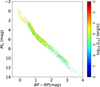 |
Fig. 1 Color-magnitude diagram of the sources, using absolute magnitude (MG) and color (BP − RP) values from Gaia DR3. The color scales with X-ray luminosity (LX), showing the relationship between stellar evolutionary status and coronal activity. |
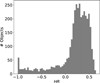 |
Fig. 2 Distribution of HRs for the analyzed sample. |
3 Analysis and results
3.1 X-ray spectral analysis
The X-ray spectral properties of the eRASS1 sources analyzed in this work are taken from the catalog presented by Gatuzz et al. (2024), where X-ray spectra were modeled using a set of simple phenomenological models commonly applied in X-ray astronomy. These models include absorbed power-law, blackbody, and optically thin thermal plasma components, as well as combinations of thermal plasma models, implemented within the xspec° spectral fitting package. In all cases, interstellar absorption along the line of sight was modeled using the tbabs model (Wilms et al. 2000). The goal of this analysis was to characterize the general spectral shape of each source and to derive key parameters such as the absorbing hydrogen column density (NH), plasma temperatures, and intrinsic X-ray fluxes.
For each source, Gatuzz et al. (2024) evaluated several candidate models and determined the best-fitting representation based on statistical criteria. In most cases, spectra of coronal sources are best described by one or two optically thin thermal plasma components, consistent with the multi-temperature structure expected from stellar coronae. The catalog provides the best-fit parameters, associated uncertainties, and both absorbed and unabsorbed flux estimates for each source. We adopted the intrinsic (unabsorbed) X-ray fluxes derived from the best-fit spectral models reported by Gatuzz et al. (2024), after having corrected for absorption using the values for the column density, NH, obtained from the spectral fits.
Figure 2 shows the hardness ratio (HR) distribution of the sources. The HR is defined as HR = (H − S )/(H + S ), where H is the unabsorbed flux in the hard X-ray band (0.5–1.0 keV) and S is the unabsorbed flux in the soft X-ray band (0.2–0.5 keV). The HR provides a proxy for the spectral shape, with higher values corresponding to harder spectra and lower values to softer emission. The distribution shows that the majority of sources lie in the HR range ∼0–0.5, indicating spectra with significant flux in both the soft and hard bands, implying that the X-ray emission of our sample stars is broadly distributed between 0.5 keV and 1.0 keV, as is typical for coronal X-ray emitters (Güdel 2004; Johnstone & Güdel 2015; Wang et al. 2020; Gatuzz et al. 2024). Then, we computed X-ray luminosities for our sample by combining the unabsorbed fluxes (FX) obtained from the spectral fits with the distances (d) derived from Gaia parallaxes. By using absorption-corrected fluxes together with distance estimates, this method accounts for the intrinsic stellar brightness in X-rays by correcting for line-of-sight absorption, thus providing a uniform estimate of the coronal emission across the sample.
3.2 From X-rays to EUV
We investigated the impact of X-ray emission on the habitability of potential planets around these stars, following the work done by Murray-Clay et al. (2009), Kubyshkina et al. (2020), Han et al. (2024), and Poppenhaeger et al. (2024). First, we computed the EUV luminosity (LEUV) in the 0.013–0.1 keV (124–95 nm) energy range by using the scaling relation from Sanz-Forcada et al. (2025):
 (2)
(2)
where CX = log LX − 27.44. LX is the X-ray luminosity, in erg s−1 and in the 0.1–2.4 keV energy range, obtained from the best-fit spectral model in ergs s−1. This scaling relation is valid only for main-sequence stars (see Sect. 2). However, it is important to emphasize that such empirical scaling laws are applied uniformly across the entire sample regardless of individual stellar age or mass. Furthermore, the atmospheric mass-loss estimates are implicitly based on a simplified H/He composition, as commonly assumed in energy-limited escape models. The combination of applying a single empirical scaling relation to all stars and assuming a simplified atmospheric composition introduces a systematic uncertainty, because it enforces a linear proportionality between X-ray and EUV luminosities. As a result, the estimates may not capture the full complexity of coronal physics across different stellar evolutionary stages.
Figures 3–6 provide complementary views of the high-energy emission of our main-sequence sample. As a reference, we also included values for the Sun and a young sun proxy from Shoda et al. (2024, their Table 1). Figure 3 presents a histogram of XUV luminosity (LXUV = log LEUV + LX). Figure 4 shows LXUV as a function of Gaia BP − RP color. For comparison, we included the Sun and κ° Ceti as a template for a Young Sun (Shoda et al. 2024) with an estimated age of ∼ 650 Myr (Airapetian et al. 2021). Figure 5 presents the relationship between LXUV and absolute magnitude (MG). We note that our sample does not include stars with LXUV ≲ 1027 erg s−1, despite our nominal LX threshold extending to 1026 erg s−1. This reflects a selection bias driven by the sensitivity limits of SRG/eROSITA and our requirement of sufficient signal for spectral analysis, which preferentially selects relatively X-ray-bright (i.e., more active) stars compared to the Sun at cycle minimum. Finally, Fig. 6 illustrates the dependence of LXUV on stellar mass, suggesting that the increase in XUV luminosity with stellar mass is most apparent for stars close to solar mass. Stellar masses used in this study were obtained directly from the Gaia DR3 astrophysical parameters table (Gaia Collaboration 2023). Specifically, we used the mass_flame parameter, which is derived from the Flux-Luminosity-Age-Mass Estimator (FLAME) module. The FLAME pipeline estimates stellar mass by comparing the Gaia observational data – including absolute luminosity derived from parallaxes and effective temperature – against standard stellar evolutionary models (Creevey et al. 2023). By combining precise Gaia astrometry with model-based evolutionary constraints, the FLAME-derived masses are therefore consistent with current stellar evolutionary tracks. These figures collectively link fundamental stellar properties with coronal activity, providing a basis for assessing the potential high-energy environment within the HZ of different stellar types.
We emphasize that the trends observed in Figs. 4 and 5 are affected by observational biases related to the eROSITA all-sky survey (eRASS) sensitivity limit. In particular, the apparent absence of F-type stars at LXUV ≲ 1030 erg s−1 (Fig. 5) likely reflects a detection bias rather than an intrinsic physical cutoff, as more luminous stars can only be detected if they exhibit sufficiently strong coronal emission. However, this trend may also be influenced by intrinsic stellar properties, since early-F stars do not generally follow the monotonic increase in XUV luminosity with stellar mass observed at later spectral types. Thus, the observed distribution likely results from a combination of observational selection effects and a change in coronal emission behavior toward earlier spectral types. This selection effect is less evident in the normalized LXUV/Lbol plane (Fig. 7). To further assess this effect, we examined the distribution of X-ray luminosity as a function of distance and found that only 98 sources lie below the nominal eRASS sensitivity limit of fX ∼ 2.5 × 10⁻¹⁴ erg cm−2 s−1 (Freund et al. 2024). Furthermore, a significant fraction of our sample lies above the canonical saturation threshold of LX/Lbol ∼ 10−3, corresponding to LXUV/Lbol ∼ 10−2.5 when accounting for the EUV contribution. This suggests that many of the detected sources are in a saturated or near-saturated regime of coronal activity.
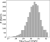 |
Fig. 3 Histogram of the XUV luminosity (LXUV) for the main-sequence sample. |
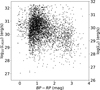 |
Fig. 4 XUV luminosity (LXUV) as a function of Gaia BP − RP color. Only sources with log(LXUV) between 1027 and 1033 erg s−1 are shown, to improve visualization. |
 |
Fig. 5 XUV luminosity (LXUV) as a function of Gaia absolute magnitude (MG). For comparison, we include the Sun and a young Sun. |
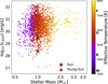 |
Fig. 6 XUV luminosity (LXUV) as a function of stellar mass. The EUV component is derived using the Sanz-Forcada et al. (2025) scaling relation. The spectral type and temperatures are also indicated. |
 |
Fig. 7 Ratio of XUV luminosity to bolometric luminosity, LXUV/Lbol, as a function of stellar effective temperature, Teff. |
3.3 HZ X-ray irradiation
Figure 7 presents the ratio of XUV luminosity to bolometric luminosity, LXUV/Lbol, as a function of stellar effective temperature, Teff. This plot reveals the dependence of stellar high-energy emission on temperature: cooler stars, typically more magnetically active, show higher LXUV/Lbol ratios, whereas hotter stars generally emit a smaller fraction of their total luminosity in the X-ray and EUV bands. Most stars in our sample exhibit LXUV/Lbol ≪ 1, which indicates that only a small fraction of their total energy is emitted in the high-energy bands, as expected for main-sequence stars.
To estimate the high-energy irradiation that a hypothetical planet would receive in the HZ of each star, we first computed the effective stellar flux defining the HZ following Kopparapu et al. (2014). The effective flux (S eff) is a function of the stellar effective temperature and can be expressed as a fourth-order polynomial relative to the solar effective temperature:
 (3)
(3)
where T⋆ = Teff − 5780 K and the coefficients Seff,⊙, a, b, c, d correspond to the inner or outer edges of the HZ depending on the chosen model. The separation of the HZ is then obtained as
 (4)
(4)
where L⊙ is the solar bolometric luminosity. Finally, the XUV flux at the HZ is calculated as
 (5)
(5)
where LXUV is XUV luminosity. The parameters used in the model correspond to the runaway greenhouse described in Table 1 in Kopparapu et al. (2014) for a 1 Earth-mass planet.
Figure 8 shows the high-energy flux that a planet would receive at the center of the HZ as a function of stellar mass (provided by Gaia). The plot illustrates that low-mass stars (M∗ < 1 M⊙) tend to expose their HZ to higher XUV fluxes due to their closer-on HZs. Conversely, more massive stars, despite having higher intrinsic XUV luminosities, have more distant HZ, which results in lower fluxes at the HZ. The majority of the computed XUV fluxes in the HZ fall between 10° and 10° erg cm−2 s−1, which is significantly larger than the present-day solar XUV flux at Earth (∼4 erg cm−2 s−1) and indicates potentially XUV-hazardous environments. The extremes correspond to very low-activity stars or highly luminous XUV emitters.
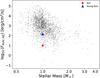 |
Fig. 8 X-ray plus EUV flux (FXUV,HZ) received at the HZ of each star as a function of stellar mass. Only sources with log(FXUV,HZ) between −1 and 6 are shown, to improve visualization. |
3.4 Exoplanet mass-loss rate
For a given planet mass and radius located within the continuous HZ (rHZ), the photo-evaporative mass loss rate (ṁ) due to high-energy stellar emission can be computed as (e.g., Owen et al. 2012; Lopez et al. 2012)
 (6)
(6)
where ρpl is the density of the planet, β is the effective XUV absorption cross section (assumed to be 2.3 as in Poppenhaeger et al. 2024), G is the gravitational constant and η is the efficiency of the atmospheric escape. This last parameter is assumed to be 0.15 as the upper limit estimated by Shematovich et al. (2014), with further discussion by Rukdee et al. (2026).
The factor K accounts for the effect of Roche lobe overflows, as described by Erkaev et al. (2007) as
 (7)
(7)
and
 (8)
(8)
with Mpl the mass of the planet, M∗ the mass of the host star, a the orbital distance between the star and the planet (taken as rHZ), and Rpl the radius of the planet.
Figure 9 shows the estimated atmospheric mass-loss rates for a hypothetical terrestrial planet (Mpl = 5.972 × 1027 g, Rpl = 6.378 × 10° cm) as a function of the HZ separation (rHZ) for each star in our sample (top panel). For comparison, observed escape rates in highly irradiated close-in exoplanets are typically in the range of 10°–1011 g s−1, which is up to 5% of its total mass per billion years (e.g., Vidal-Madjar et al. 2003; Lecavelier Des Etangs et al. 2010; Ehrenreich et al. 2015; Ginzburg et al. 2018; Spake et al. 2018; Cubillos et al. 2020; Hazra 2025), consistent with our model predictions for highly irradiated systems.
The color-coding in Fig. 9 represents the stellar mass. We observe a general decrease in the mass-loss rates as stellar mass increases. For stars with M∗ > 1.5 M⊙, the HZs are located at greater orbital separations (Gallet et al. 2017), which significantly attenuates the incident XUV flux and results in more moderate mass-loss rates, typically below 10° g s−1. In contrast, low-mass stars (M∗ < 1.0 M⊙) exhibit a much broader distribution of mass-loss rates, spanning over five orders of magnitude. While some low-mass stars provide relatively benign environments, a significant subset drives extreme escape rates exceeding 1010 g s−1 due to high XUV irradiation levels (FXUV,HZ), as indicated by the color scale. These results suggest that stars with M∗ > 1.5 M⊙ are more favorable for the long-term retention of secondary atmospheres on HZ planets. Conversely, planets orbiting low-mass stars – particularly those in active or young phases – face a higher risk of total atmospheric erosion, potentially rendering their HZs less hospitable despite the favorable thermal conditions.
We stress that the mass-loss rates derived here should be interpreted with caution. In this work, we adopted an Earth-like density as a reference case to provide an order-of-magnitude estimate of the potential impact of stellar XUV irradiation, rather than a self-consistent description of atmospheric escape for rocky planets. An additional limitation is that our estimates are based on present-day stellar XUV luminosities, whereas atmospheric escape is expected to have been more efficient during earlier evolutionary phases when stellar activity levels were significantly higher. Therefore, our results should be viewed as indicative of relative trends across the stellar sample and as a proxy for defining potential hazard zones of high-energy irradiation, rather than as precise predictions of atmospheric evolution for HZ terrestrial planets.
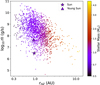 |
Fig. 9 Calculated photo-evaporative mass-loss rates for a theoretical Earth-like planet orbiting the sample of stars as a function of the HZ separation (rHZ). Each data point represents a unique star–planet combination. The color scale indicates the stellar mass of the incident star. |
3.5 Mapping local hazard zones
Figure 10 shows the normalized XUV flux ratio, FXUV,HZ/FHZ, in the Galactic plane for our sample of stars. This ratio quantifies the fraction of stellar high-energy emission relative to the total bolometric flux at the HZ. To construct these 2D maps, we binned the stellar sample in cylindrical coordinates, defined as (R, ϕ, Z) with
 (9)
(9)
where (X, Y, Z) are the Cartesian Galactocentric coordinates. The spatial distribution of our sample in Galactocentric coordinates is restricted to the southern Galactic hemisphere (Y ≤ 0). To construct these 2D maps, we binned the stellar sample in cylindrical coordinates (R, Z), where  is the radial Galactocentric distance. The average XUV flux in each bin was computed by weighting the logarithmic values by the number of stars per bin. This approach accounts for the nonuniform stellar distribution and provides a representative measure of the typical irradiation environment in each region. The map was constructed using bins of 30 pc in both the radial and vertical directions.
It is important to note that such maps are located in the solar neighborhood, within a heliocentric distance range of 4.47−1104.2 pc (R = 8.2−8.8 kpc in Galactocentric coordinates). Figure 11 displays the star counts per bin on a logarithmic scale to highlight the sampling significance. As expected for a flux-limited sample, the highest statistical significance is concentrated near the Sun (R ≈ 8.5 kpc, Z ≈ 0 kpc), where the sampling density is highest. Conversely, isolated pixels at larger heliocentric distances (lower Z or extreme R) contain significantly fewer objects. These outer regions are more susceptible to Malmquist bias – where only the most X-ray luminous stars are detected at large distances – and Poissonian noise. The central, high-density region of the map provides the most robust representation of the typical irradiation environment.
Figure 10 shows that most values are clustered around log10(FXUV,HZ/FHZ) = (−2.5, −1.5), while the plotted range is chosen to enhance visualization. Areas with higher ratios indicate environments where XUV irradiation is proportionally stronger, suggesting potentially harsher conditions for planetary atmospheres. These maps provide a Galactic-scale view of hazard zones, identifying regions where high-energy stellar radiation could significantly influence habitability. For reference, the Sun XUV flux in its HZ is FXUV,HZ,⊙ ∼ 4 erg cm−2 s−1, while the bolometric flux at 1 AU is FHZ,⊙ ∼ 1.36 × 10° erg cm−2 s−1, giving a ratio FXUV,HZ/FHZ ∼ 3 × 10⁻⁶. As expected, most stars in our sample are significantly more XUV-active than the Sun.
The observed outliers, particularly those showing enhanced FXUV,HZ/FHZ ratios, were examined for potential associations with young moving groups or known stellar clusters. While the spatial distribution of these high-activity bins is broadly consistent with the direction of young local associations such as the Orion complex (187.5◦ < l < 218◦, −25◦ < b < −4◦, as defined by Rezaei Kh. et al. 2018) or various moving groups, the low occupancy of these bins (typically N < 3 stars) suggests they are highly sensitive to individual high-activity outliers. Consequently, while these features hint at the presence of age-dependent hazard zones tied to recent star-formation history, they likely represent the tail of the X-ray luminosity function rather than a systematic Galactic trend.
To further investigate the nature of the high-FXUV,HZ/FHZ outliers forming the apparent high-|Z| tail, we identified the individual sources contributing to these bins. In total, 19 stars were found in this region. Cross-matching their coordinates with the Set of Identifications, Measurements and Bibliography for Astronomical Data (SIMBAD) did not support an association with the Orion complex or any known nearby star-forming region. Instead, these objects appear to be a heterogeneous population, including eclipsing binaries, high proper-motion stars, and RR Lyrae variables. The lack of association with known star-forming regions, together with the heterogeneous nature of these sources, suggests that the enhanced XUV flux ratios observed in these bins are not linked to a coherent young stellar population, but rather arise from intrinsically X-ray-active or variable sources. Further spectroscopic age-dating of the stars in these specific bins would be required to confirm whether they belong to coherent kinematic structures. The combination of the small number of objects per bin and their heterogeneous classifications indicates that the “yellow tail” is dominated by statistical fluctuations and selection effects, rather than tracing a genuine Galactic-scale structure or recent star-forming event.
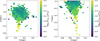 |
Fig. 10 Left: map of the normalized XUV flux in the HZ, FXUV,HZ/FHZ, in the Galactic R-Z plane. Right: map of the normalized XUV flux in the HZ, FXUV,HZ/FHZ, in the Galactic X-Y plane. |
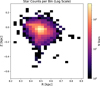 |
Fig. 11 Stellar density distribution in the Galactic plane for the studied sample. The map shows the number of stars per 30 × 30 pc bin on a logarithmic scale. The highest statistical significance is concentrated in the solar neighborhood (R ≈ 8.5 kpc, Z ≈ 0 kpc). Isolated pixels at larger heliocentric distances (low Z) represent low-count bins (N < 10). |
4 Discussion
Our study provides an estimation of atmospheric mass-loss rates for exoplanets, focusing on the energy-limited escape mechanism. Our results are broadly consistent with previous studies, confirming that the energy-limited approximation is a useful tool for estimating mass-loss rates in many cases. Ehrenreich & Désert (2011) estimated mass-loss rates for transiting exoplanets, finding values ranging from 10° to 1013 g s−1 under various assumptions. Similarly, Krenn et al. (2021) critically assessed the applicability of this approximation, concluding that it provides correct order-of-magnitude estimates for approximately 76% of planets. However, for planets with very low or very high gravitational potentials, or those subject to high equilibrium temperatures and strong irradiation fluxes, the energy-limited approximation can deviate from hydrodynamic simulation predictions by up to three orders of magnitude in individual cases (e.g., Kubyshkina et al. 2018; Krenn et al. 2021; Caldiroli et al. 2022). This work further highlights the complex relationship between the incident X-ray flux on the planet, and its atmospheric mass-loss rate.
Understanding atmospheric mass loss is crucial for modeling the long-term evolution of exoplanetary atmospheres. Previous works (e.g., Sanz-Forcada et al. 2011; Owen et al. 2012; Lopez & Fortney 2014; Sanz-Forcada et al. 2025) have shown that XUV-driven mass loss can significantly alter the atmospheric composition and survival of close-in planets around active stars. Foster et al. (2022) conducted a comprehensive study utilizing eROSITA data to estimate X-ray and EUV irradiation fluxes and corresponding mass-loss rates for 287 known exoplanets. Their analysis combined stellar X-ray luminosities measured with eROSITA with empirical scaling relations to estimate the EUV emission and the resulting XUV flux incident on the planetary atmospheres. They found that many close-in exoplanets are subject to intense high-energy irradiation capable of driving substantial atmospheric escape. While that study focused on the irradiation and evaporation rates of known exoplanets, the present work adopts a complementary approach by analyzing the XUV radiation environment of a large sample of main-sequence stars detected with eROSITA. Instead of targeting specific planetary systems, we investigated the high-energy conditions within the HZs of these stars and estimated atmospheric mass-loss rates for hypothetical Earth-like planets. This approach allowed us to characterize the broader stellar XUV environment relevant for planetary habitability in the solar neighborhood.
Our findings build upon this body of work by providing updated mass-loss rates for a large sample of main-sequence stars, using an extensive catalog of coronal sources. We stress that our sample is flux-limited and thus biased toward the most X-ray luminous stars, which naturally results in higher average XUV fluxes compared to a solar-like star. For reference, the present-day XUV flux at the solar HZ is ∼4 erg cm−2 s−1, while our sample exhibits values ranging from 10° to 10° erg cm−2 s−1. It is important to note that coronal activity decreases with stellar age (Ribas et al. 2005; Tu et al. 2015; Johnstone et al. 2021), and most of the sources in our sample are likely young, magnetically active stars. At comparable ages, the young Sun is also believed to have emitted significantly stronger XUV radiation than today, by up to two orders of magnitude (Ribas et al. 2005; Claire et al. 2012). This evolutionary context suggests that our high flux levels are consistent with expectations for young stellar populations and highlight the temporal dependence of atmospheric erosion processes. The maps we present therefore provide a first-order view of the local distribution of potentially hazardous radiation environments, illustrating where exoplanetary atmospheres may be most strongly affected by stellar XUV irradiation. We find that the ratio LXUV/Lbol is generally higher for cooler stars, aligning with the saturation levels observed in early M dwarfs by Jackson et al. (2012) and the XUV-scaling laws derived by Sanz-Forcada et al. (2011). Specifically, our results confirm that stars in the higher-activity regime (LXUV/Lbol ∼ 10−3) are predominantly located in low-Z regions of the Galactic plane, suggesting a younger, more active population similar to the “active” branch of the local X-ray luminosity function discussed by Schmitt & Liefke (2004). By mapping these values in 3D, we extended these local activity-color relations to a Galactic-scale view of hazard zones. While the Sun occupies a relatively quiescent position in this distribution, the majority of our sample exhibits irradiation environments that are significantly more extreme, highlighting the importance of high-energy stellar evolution in shaping planetary habitability across the Galaxy.
While the energy-limited model provides a valuable first-order estimate, it does not account for detailed hydrodynamic processes, magnetic fields, or core-powered mass-loss mechanisms, which can become significant in extreme irradiation environments (Owen & Wu 2016; Thorngren & Fortney 2018). Future work should incorporate these effects to improve the accuracy of mass-loss predictions, particularly for hot Jupiters and highly irradiated super-Earths. The unprecedented data from eROSITA provides a critical foundation for these future studies, offering a robust dataset to constrain stellar XUV fluxes and refine our understanding of exoplanetary atmospheric escape.
5 Conclusion
In this work, we utilized the extensive all-sky X-ray survey data from SRG/eROSITA to study stellar high-energy radiation and its impact on exoplanet habitability. By combining our robust sample of 3750 main-sequence stars with Gaia astrometry, we computed XUV luminosities and fluxes at the HZ. Our analysis reveals that the majority of stars in our sample are significantly more XUV-active than the Sun, with HZ fluxes ranging from 10° to 10° erg cm−2 s−1. We find that cooler, more active stars exhibit a higher ratio of XUV to bolometric luminosity (LXUV/Lbol), and we created Galactic-scale maps that identify hazard zones where XUV irradiation is highest. We modeled atmospheric mass-loss ratios for Earth-like planets located in the HZ for each star, which showed the importance of the incident X-ray flux in the photo-evaporation process. These results highlight the critical role of stellar high-energy emission in planetary atmospheric evolution and emphasize the need for direct XUV observations to fully understand the long-term habitability of exoplanets.
Data availability
Table 1 is available at the CDS via https://cdsarc.cds.unistra.fr/viz-bin/cat/J/A+A/710/A273
Acknowledgements
This work is based on data from eROSITA, the soft X-ray instrument aboard SRG, a joint Russian-German science mission supported by the Russian Space Agency (Roskosmos), in the interests of the Russian Academy of Sciences represented by its Space Research Institute (IKI), and the Deutsches Zentrum für Luft- und Raumfahrt (DLR). The SRG spacecraft was built by Lavochkin Association (NPOL) and its subcontractors, and is operated by NPOL with support from the Max Planck Institute for Extraterrestrial Physics (MPE). The development and construction of the eROSITA X-ray instrument was led by MPE, with contributions from the Dr. Karl Remeis Observatory Bamberg & ECAP (FAU Erlangen-Nuernberg), the University of Hamburg Observatory, the Leibniz Institute for Astrophysics Potsdam (AIP), and the Institute for Astronomy and Astrophysics of the University of Tübingen, with the support of DLR and the Max Planck Society. The Argelander Institute for Astronomy of the University of Bonn and the Ludwig Maximilians Universität Munich also participated in the science preparation for eROSITA. This research was carried out on the High Performance Computing resources of the cobra cluster at the Max Planck Computing and Data Facility (MPCDF) in Garching operated by the Max Planck Society (MPG). The eROSITA data shown here were processed using the eSASS software system developed by the German eROSITA consortium. This research was carried out on the High Performance Computing resources of the cobra cluster at the Max Planck Computing and Data Facility (MPCDF) in Garching operated by the Max Planck Society (MPG).
References
- Airapetian, V. S., Jin, M., Lüftinger, T., et al. 2021, ApJ, 916, 96 [NASA ADS] [CrossRef] [Google Scholar]
- Allart, R., Bourrier, V., Lovis, C., et al. 2018, Science, 362, 1384 [Google Scholar]
- Baraffe, I., & Chabrier, G. 2010, A&A, 521, A44 [NASA ADS] [CrossRef] [EDP Sciences] [Google Scholar]
- Brunner, H., Liu, T., Lamer, G., et al. 2022, A&A, 661, A1 [NASA ADS] [CrossRef] [EDP Sciences] [Google Scholar]
- Caldiroli, A., Haardt, F., Gallo, E., et al. 2022, A&A, 663, A122 [NASA ADS] [CrossRef] [EDP Sciences] [Google Scholar]
- Caramazza, M., Stelzer, B., Magaudda, E., et al. 2023, A&A, 676, A14 [NASA ADS] [CrossRef] [EDP Sciences] [Google Scholar]
- Claire, M. W., Sheets, J., Cohen, M., et al. 2012, ApJ, 757, 95 [Google Scholar]
- Cohen, O., Ma, Y., Drake, J. J., et al. 2015, ApJ, 806, 41 [NASA ADS] [CrossRef] [Google Scholar]
- Creevey, O. L., Sordo, R., Pailler, F., et al. 2023, A&A, 674, A26 [NASA ADS] [CrossRef] [EDP Sciences] [Google Scholar]
- Cubillos, P. E., Fossati, L., Koskinen, T., et al. 2020, AJ, 159, 111 [Google Scholar]
- Dong, C., Lingam, M., Ma, Y., & Cohen, O. 2017, ApJ, 837, L26 [NASA ADS] [CrossRef] [Google Scholar]
- Ehrenreich, D., & Désert, J. M. 2011, A&A, 529, A136 [NASA ADS] [CrossRef] [EDP Sciences] [Google Scholar]
- Ehrenreich, D., Bourrier, V., Wheatley, P. J., et al. 2015, Nature, 522, 459 [Google Scholar]
- Erkaev, N. V., Kulikov, Y. N., Lammer, H., et al. 2007, A&A, 472, 329 [NASA ADS] [CrossRef] [EDP Sciences] [Google Scholar]
- Fortney, J. J., & Nettelmann, N. 2010, Space Sci. Rev., 152, 423 [CrossRef] [Google Scholar]
- Foster, G., Poppenhaeger, K., Ilic, N., & Schwope, A. 2022, A&A, 661, A23 [NASA ADS] [CrossRef] [EDP Sciences] [Google Scholar]
- France, K., Froning, C. S., Linsky, J. L., et al. 2013, ApJ, 763, 149 [Google Scholar]
- Freund, S., Czesla, S., Robrade, J., Schneider, P. C., & Schmitt, J. H. M. M. 2022, A&A, 664, A105 [NASA ADS] [CrossRef] [EDP Sciences] [Google Scholar]
- Freund, S., Czesla, S., Predehl, P., et al. 2024, A&A, 684, A121 [NASA ADS] [CrossRef] [EDP Sciences] [Google Scholar]
- Gaia Collaboration (Brown, A. G. A., et al.) 2021, A&A, 649, A1 [NASA ADS] [CrossRef] [EDP Sciences] [Google Scholar]
- Gaia Collaboration (Vallenari, A., et al.) 2023, A&A, 674, A1 [NASA ADS] [CrossRef] [EDP Sciences] [Google Scholar]
- Gallet, F., Charbonnel, C., Amard, L., et al. 2017, A&A, 597, A14 [NASA ADS] [CrossRef] [EDP Sciences] [Google Scholar]
- Gatuzz, E., Wilms, J., Zainab, A., et al. 2024, A&A, 688, A207 [NASA ADS] [CrossRef] [EDP Sciences] [Google Scholar]
- Ginzburg, S., Schlichting, H. E., & Sari, R. 2018, MNRAS, 476, 759 [Google Scholar]
- Güdel, M. 2004, A&A Rev., 12, 71 [Google Scholar]
- Han, H., Wang, S., Zheng, C., et al. 2024, ApJS, 273, 8 [Google Scholar]
- Hazra, G. 2025, Rev. Mod. Plasma Phys., 9, 18 [Google Scholar]
- Jackson, A. P., Davis, T. A., & Wheatley, P. J. 2012, MNRAS, 422, 2024 [Google Scholar]
- Johnstone, C. P., & Güdel, M. 2015, A&A, 578, A129 [NASA ADS] [CrossRef] [EDP Sciences] [Google Scholar]
- Johnstone, C. P., Bartel, M., & Güdel, M. 2021, A&A, 649, A96 [EDP Sciences] [Google Scholar]
- Kopparapu, R. K., Ramirez, R. M., SchottelKotte, J., et al. 2014, ApJ, 787, L29 [Google Scholar]
- Krenn, A. F., Fossati, L., Kubyshkina, D., & Lammer, H. 2021, A&A, 650, A94 [NASA ADS] [CrossRef] [EDP Sciences] [Google Scholar]
- Kubyshkina, D., Fossati, L., Erkaev, N. V., et al. 2018, ApJ, 866, L18 [NASA ADS] [CrossRef] [Google Scholar]
- Kubyshkina, D., Vidotto, A. A., Fossati, L., & Farrell, E. 2020, MNRAS, 499, 77 [Google Scholar]
- Kulow, J. R., France, K., Linsky, J., & Loyd, R. O. P. 2014, ApJ, 786, 132 [Google Scholar]
- Lecavelier Des Etangs, A., Ehrenreich, D., Vidal-Madjar, A., et al. 2010, A&A, 514, A72 [NASA ADS] [CrossRef] [EDP Sciences] [Google Scholar]
- Lopez, E. D., & Fortney, J. J. 2014, ApJ, 792, 1 [Google Scholar]
- Lopez, E. D., Fortney, J. J., & Miller, N. 2012, ApJ, 761, 59 [Google Scholar]
- Magaudda, E., Stelzer, B., Raetz, S., et al. 2022, A&A, 661, A29 [NASA ADS] [CrossRef] [EDP Sciences] [Google Scholar]
- Mayor, M., & Queloz, D. 1995, Nature, 378, 355 [Google Scholar]
- Merloni, A., Lamer, G., Liu, T., et al. 2024, A&A, 682, A34 [NASA ADS] [CrossRef] [EDP Sciences] [Google Scholar]
- Monsch, K., Ercolano, B., Picogna, G., Preibisch, T., & Rau, M. M. 2019, MNRAS, 483, 3448 [Google Scholar]
- Murray-Clay, R. A., Chiang, E. I., & Murray, N. 2009, ApJ, 693, 23 [Google Scholar]
- Nortmann, L., Pallé, E., Salz, M., et al. 2018, Science, 362, 1388 [Google Scholar]
- Oklopčić, A., & Hirata, C. M. 2018, ApJ, 855, L11 [Google Scholar]
- Owen, J. E., & Adams, F. C. 2014, MNRAS, 444, 3761 [Google Scholar]
- Owen, J. E., & Wu, Y. 2016, ApJ, 817, 107 [NASA ADS] [CrossRef] [Google Scholar]
- Owen, J. E., Clarke, C. J., & Ercolano, B. 2012, MNRAS, 422, 1880 [Google Scholar]
- Pecaut, M. J., & Mamajek, E. E. 2013, ApJS, 208, 9 [Google Scholar]
- Pecaut, M. J., Mamajek, E. E., & Bubar, E. J. 2012, ApJ, 746, 154 [Google Scholar]
- Poppenhaeger, K., Schmitt, J. H. M. M., & Wolk, S. J. 2013, ApJ, 773, 62 [Google Scholar]
- Poppenhaeger, K., Ketzer, L., Ilic, N., et al. 2024, A&A, 689, A188 [NASA ADS] [CrossRef] [EDP Sciences] [Google Scholar]
- Predehl, P., Andritschke, R., Arefiev, V., et al. 2021, A&A, 647, A1 [EDP Sciences] [Google Scholar]
- Rezaei Kh., S., Bailer-Jones, C. A. L., Schlafly, E. F., & Fouesneau, M. 2018, A&A, 616, A44 [NASA ADS] [CrossRef] [EDP Sciences] [Google Scholar]
- Ribas, I., Guinan, E. F., Güdel, M., & Audard, M. 2005, ApJ, 622, 680 [Google Scholar]
- Rukdee, S., Güdel, M., Vilović, I., et al. 2026, A&A, 707, A219 [NASA ADS] [CrossRef] [EDP Sciences] [Google Scholar]
- Salz, M., Schneider, P. C., Fossati, L., et al. 2019, A&A, 623, A57 [NASA ADS] [CrossRef] [EDP Sciences] [Google Scholar]
- Sanz-Forcada, J., Micela, G., Ribas, I., et al. 2011, A&A, 532, A6 [NASA ADS] [CrossRef] [EDP Sciences] [Google Scholar]
- Sanz-Forcada, J., López-Puertas, M., Lampón, M., et al. 2025, A&A, 693, A285 [NASA ADS] [CrossRef] [EDP Sciences] [Google Scholar]
- Schmitt, J. H. M. M., & Liefke, C. 2004, A&A, 417, 651 [NASA ADS] [CrossRef] [EDP Sciences] [Google Scholar]
- Schneider, P. C., Freund, S., Czesla, S., et al. 2022, A&A, 661, A6 [NASA ADS] [CrossRef] [EDP Sciences] [Google Scholar]
- Shematovich, V. I., Ionov, D. E., & Lammer, H. 2014, A&A, 571, A94 [NASA ADS] [CrossRef] [EDP Sciences] [Google Scholar]
- Shoda, M., Namekata, K., & Takasao, S. 2024, A&A, 691, A152 [NASA ADS] [CrossRef] [EDP Sciences] [Google Scholar]
- Spake, J. J., Sing, D. K., Evans, T. M., et al. 2018, Nature, 557, 68 [Google Scholar]
- Thorngren, D. P., & Fortney, J. J. 2018, AJ, 155, 214 [Google Scholar]
- Truemper, J. 1982, Adv. Space Res., 2, 241 [Google Scholar]
- Tu, L., Johnstone, C. P., Güdel, M., & Lammer, H. 2015, A&A, 577, L3 [NASA ADS] [CrossRef] [EDP Sciences] [Google Scholar]
- Vidal-Madjar, A., Lecavelier des Etangs, A., Désert, J. M., et al. 2003, Nature, 422, 143 [Google Scholar]
- Wang, S., Bai, Y., He, L., & Liu, J. 2020, ApJ, 902, 114 [NASA ADS] [CrossRef] [Google Scholar]
- Watson, A. J., Donahue, T. M., & Walker, J. C. G. 1981, Icarus, 48, 150 [NASA ADS] [CrossRef] [Google Scholar]
- Wilms, J., Allen, A., & McCray, R. 2000, ApJ, 542, 914 [Google Scholar]
- Yelle, R. V. 2004, Icarus, 170, 167 [NASA ADS] [CrossRef] [Google Scholar]
All Figures
|
Fig. 1 Color-magnitude diagram of the sources, using absolute magnitude (MG) and color (BP − RP) values from Gaia DR3. The color scales with X-ray luminosity (LX), showing the relationship between stellar evolutionary status and coronal activity. |
| In the text | |
|
Fig. 2 Distribution of HRs for the analyzed sample. |
| In the text | |
|
Fig. 3 Histogram of the XUV luminosity (LXUV) for the main-sequence sample. |
| In the text | |
|
Fig. 4 XUV luminosity (LXUV) as a function of Gaia BP − RP color. Only sources with log(LXUV) between 1027 and 1033 erg s−1 are shown, to improve visualization. |
| In the text | |
|
Fig. 5 XUV luminosity (LXUV) as a function of Gaia absolute magnitude (MG). For comparison, we include the Sun and a young Sun. |
| In the text | |
|
Fig. 6 XUV luminosity (LXUV) as a function of stellar mass. The EUV component is derived using the Sanz-Forcada et al. (2025) scaling relation. The spectral type and temperatures are also indicated. |
| In the text | |
|
Fig. 7 Ratio of XUV luminosity to bolometric luminosity, LXUV/Lbol, as a function of stellar effective temperature, Teff. |
| In the text | |
|
Fig. 8 X-ray plus EUV flux (FXUV,HZ) received at the HZ of each star as a function of stellar mass. Only sources with log(FXUV,HZ) between −1 and 6 are shown, to improve visualization. |
| In the text | |
|
Fig. 9 Calculated photo-evaporative mass-loss rates for a theoretical Earth-like planet orbiting the sample of stars as a function of the HZ separation (rHZ). Each data point represents a unique star–planet combination. The color scale indicates the stellar mass of the incident star. |
| In the text | |
|
Fig. 10 Left: map of the normalized XUV flux in the HZ, FXUV,HZ/FHZ, in the Galactic R-Z plane. Right: map of the normalized XUV flux in the HZ, FXUV,HZ/FHZ, in the Galactic X-Y plane. |
| In the text | |
|
Fig. 11 Stellar density distribution in the Galactic plane for the studied sample. The map shows the number of stars per 30 × 30 pc bin on a logarithmic scale. The highest statistical significance is concentrated in the solar neighborhood (R ≈ 8.5 kpc, Z ≈ 0 kpc). Isolated pixels at larger heliocentric distances (low Z) represent low-count bins (N < 10). |
| In the text | |
Current usage metrics show cumulative count of Article Views (full-text article views including HTML views, PDF and ePub downloads, according to the available data) and Abstracts Views on Vision4Press platform.
Data correspond to usage on the plateform after 2015. The current usage metrics is available 48-96 hours after online publication and is updated daily on week days.
Initial download of the metrics may take a while.