


| Issue |
A&A
Volume 710, June 2026
|
|
|---|---|---|
| Article Number | A156 | |
| Number of page(s) | 13 | |
| Section | Extragalactic astronomy | |
| DOI | https://doi.org/10.1051/0004-6361/202558801 | |
| Published online | 12 June 2026 | |
H I-bearing dark galaxy predictions from constrained Local Group simulations: How many and where to find them
1
Departamento de Astrofísica, Universidad de La Laguna, E-38200 La Laguna, Tenerife, Spain
2
Instituto de Astrofísica de Canarias, Calle Via Láctea s/n, E-38206 La Laguna, Tenerife, Spain
3
Leibniz Institut für Astrophysik Potsdam (AIP), An der Sternwarte 16, D-14482 Potsdam, Germany
4
Facultad de Física, Universidad de Sevilla, Avda. Reina Mercedes s/n, Campus de Reina Mercedes, E-41012 Sevilla, Spain
5
INAF – Osservatorio di Astrofisica e Scienza dello Spazio di Bologna, Via Gobetti 93/3, I-40129 Bologna, Italy
6
Departamento de Física Teórica, Módulo 15, Facultad de Ciencias, Universidad Autónoma de Madrid, 28049 Madrid, Spain
7
Centro de Investigación Avanzada en Física Fundamental (CIAFF), Facultad de Ciencias, Universidad Autónoma de Madrid, 28049 Madrid, Spain
8
International Centre for Radio Astronomy Research, University of Western Australia, 35 Stirling Highway, Crawley, Western Australia, 6009, Australia
★ Corresponding authors: This email address is being protected from spambots. You need JavaScript enabled to view it.
; This email address is being protected from spambots. You need JavaScript enabled to view it.
Received:
27
December
2025
Accepted:
1
April
2026
Abstract
Context. Dark galaxies are small, dark matter-dominated haloes whose gas remains in hydrostatic and thermal equilibrium and has never formed stars. These systems are of particular interest because they represent a strong prediction of the Lambda cold dark matter (ΛCDM) model. As of today, only a few dark galaxy candidates have been detected so far, the most intriguing of which being Cloud-9.
Aims. Using several state-of-the-art hydrodynamical simulations, we aim to predict the abundance of dark galaxies within our Local Group, characterise their physical properties, and provide guidance for their potential observational detection.
Methods. We analyse Local Group simulations with constrained initial conditions, each run with different codes, implementing different baryonic physics, feedback prescriptions, and employing two distinct values of star-formation density threshold, nth = 0.13 and 10 cm−3, to select samples of dark and bright galaxies harboured in haloes of similar mass.
Results. We demonstrate that dark galaxies exist in all such simulations, though their number is larger in simulations that use a higher, more realistic nth. These galaxies, whose gas remains diffuse and never forms stars, predominantly inhabit less-concentrated, higher-spin dark matter haloes than their luminous counterparts. Dark galaxies are typically found in low-density regions at the outskirts of the Local Group. Their formation and evolution across redshift indicate that both the dark matter and gas densities in the surroundings of dark galaxies were consistently lower than those found around bright galaxies, making them less susceptible to interactions, mergers, or gas inflows. We estimate that up to eight dark galaxies should be detectable in H I emission within 2.5 Mpc of the Milky Way, with the FAST radio telescope, accounting for its sky coverage and minimum H I mass and column density.
Conclusions. Current hydrodynamical simulations of galaxies, combined with upcoming H I surveys, will offer a direct and powerful test of ΛCDM through their ability to predict and measure properties of dark galaxies within and beyond the Local Group.
Key words: methods: numerical / galaxies: dwarf / galaxies: evolution / galaxies: formation / Local Group / dark matter
© The Authors 2026
 Open Access article, published by EDP Sciences, under the terms of the Creative Commons Attribution License (https://creativecommons.org/licenses/by/4.0), which permits unrestricted use, distribution, and reproduction in any medium, provided the original work is properly cited.
This article is published in open access under the Subscribe to Open model. This email address is being protected from spambots. You need JavaScript enabled to view it. to support open access publication.
1. Introduction
Within the Lambda cold dark matter (ΛCDM) model, galaxies form hierarchically through the gravitational collapse of small dark matter (DM) structures (White & Rees 1978), which then merge to form larger systems. This progressive growth of structures builds the DM haloes in which galaxies are embedded, enabling them to accrete gas that later cools and to create stars. In this framework of cold DM bottom-up assembly of structures, we expect a large number of low-mass DM haloes. Some of these haloes may have a low stellar-mass content or even be starless. These objects are called dark galaxies, due to their expected DM-dominated nature (e.g. Trentham et al. 2001; Kent et al. 2007).
Being such a strong prediction of the ΛCDM model, finding dark galaxies has been one of the main objectives of world-class radio telescopes such as the Arecibo radio telescope, through its Arecibo Legacy Fast ALFA (ALFALFA) Survey (Giovanelli et al. 2005; Haynes et al. 2011), and the more recent Five-Hundred-Meter Aperture Spherical Telescope (FAST; Zhang et al. 2024).
Theoretically, it has been demonstrated that only structures with masses above a certain redshift-dependent critical mass are able to retain gas in their potential well to form stars and become luminous galaxies (e.g. Hoeft et al. 2006; Okamoto et al. 2008; Benitez-Llambay & Frenk 2020). This critical mass is Mcrit ≈ 5 × 10⁹ M⊙ to the present day (Benitez-Llambay & Frenk 2020; Nebrin et al. 2023), and it depends on the time at which reionisation took place and on the mass assembly rate of each galaxy. Thus, reionisation plays an essential role in the galaxy evolution process, as it can quench and avoid star formation (SF) in small haloes, by photoheating and removing their gas (e.g. Benítez-Llambay et al. 2017). Those small haloes that are able to retain cold and dense gas to form neutral hydrogen (H I) at their centres but are affected by cosmic reionisation in such a manner (i.e. they currently have zero or few stars) have been dubbed REionisation-limited H I clouds or RELHICS (Benítez-Llambay et al. 2017). These cover a halo mass range between ∼108 M⊙ and ∼5 × 10⁹ M⊙, and are equivalent to the mini-haloes initially proposed by Rees (1986) and Ikeuchi (1986).
Due to their nature, RELHICs are challenging to observe. In fact, there are no confirmed dark galaxies, but there are a few candidates like Cloud-9 (Zhou et al. 2023; Benitez-Llambay & Navarro 2023), or more recently, Candidate Dark Galaxy-2 or CDG-2 (Li et al. 2025b), among others (e.g. Minchin et al. 2005; van Loon et al. 2009; Leisman et al. 2021; Xu et al. 2023; Liu et al. 2025). As for Cloud-9, these objects can potentially be detected as sources of H I 21 cm emission without an apparent stellar counterpart, using instruments such as FAST.
Cloud-9 is a potential starless dark galaxy, detected as an H I cloud close to M94, and appears to be devoid of a stellar component within the Dark Energy Spectroscopic Instrument Legacy Imaging Survey (DESI-LS) surface brightness limit (Martínez-Delgado et al. 2023). It is a gas-rich object with MH I ≈ 106 M⊙ (Karunakaran & Spekkens 2024; Benítez-Llambay et al. 2024) and DM halo mass of M200 ∼ 5 × 10⁹ M⊙ (Zhou et al. 2023; Benitez-Llambay & Navarro 2023). Following the predictions of Benítez-Llambay et al. (2017), it presents a gas temperature of T ∼ 2 × 10⁴ K. Cloud-9 is estimated to be located at a distance of d ∼ 4.7 Mpc (upper limit of ∼10 Mpc) and has a halo concentration of cNFW ∼ 13 (Benitez-Llambay & Navarro 2023). Moreover, a recent study by Anand et al. (2025) confirms Cloud-9 as the first detected RELHIC. Using deep Hubble Space Telescope (HST) Advanced Camera for Surveys (ACS) imaging, the authors derive a new upper limit on its stellar mass of ∼103.5 M⊙.
The CDG-2 is also a recently discovered prospective candidate for an almost dark ultra-diffuse galaxy, first identified by Li et al. (2025a) through the faint and diffuse emission of its population of globular clusters with HST. It is located in the Perseus cluster, at a distance of 75 Mpc, and has a total stellar mass of M* ≈ 1.2 × 10⁷ M⊙, and a halo mass of Mhalo ≈ 2 − 5.7 × 10¹⁰ M⊙, which indicates that it resides in a massive DM halo (Li et al. 2025b).
In this context, numerical simulations developed within ΛCDM are an important tool that can help us test results and make predictions on the nature of dark galaxies. In particular, simulations of the Local Group are key to understanding the main drivers for the formation and evolution of the galaxies residing within, as well as their environmental dependence.
In the work of Benítez-Llambay et al. (2017), for example, they analysed the properties of RELHICs in a Local Group environment with APOSTLE cosmological zoom-in simulations (Fattahi et al. 2016; Sawala et al. 2016). Their results showed that these systems harbour gas and reside beyond 500 kpc from the Milky Way (MW), with most of their gas in an ionised state, except for a small nearly spherical H I core. Moreover, the gas in these systems was found to be in hydrostatic equilibrium with the underlying Navarro-Frenk-White halo (NFW; Navarro et al. 1996, 1997), and in thermal equilibrium with the cosmic UV radiation background. However, the original APOSTLE simulations of the Local Group were affected by an overproduction of stars at a fixed halo mass (Sawala et al. 2016), which casts doubts about the predicted number of dark galaxies found within them.
More recently, Lee et al. (2024) used simulations from the IllustrisTNG project (e.g. Nelson et al. 2019; Pillepich et al. 2019) to explore the nature of dark galaxies. Within the TNG50 volume, they identify dark galaxies with DM halo masses ∼109 h−1 M⊙ and stellar-to-total-mass ratios M★/Mtot < 10−4 at z = 0. They find that dark galaxies live mainly in voids and tend to be larger in size and have larger spin parameters than their luminous counterparts (see also Jimenez & Heavens 2020). However, the TNG50 simulation shares a similar issue of overcooling with the APOSTLE simulations. More specifically, below a halo mass of 1011 M⊙, most dwarf galaxies tend to overproduce stars compared to the expected abundance-matching relations (Moster et al. 2013; Brook et al. 2014; Girelli et al. 2020). In addition, Lee et al. (2024) do not require their dark galaxies sample to explicitly contain gas, thus making it difficult to use their predictions in the light of upcoming H I surveys. The tendency of dark galaxies to live in low density regions has also been recently explored observationally in Kwon et al. (2025), who study the properties of a selection of prospective dark galaxy candidates from the ALFALFA Survey (Haynes et al. 2018).
In this work, we move forward by studying the number, distribution, and characteristics of dark galaxies arising in different sets of zoom-in Local Group simulations, and offer concrete predictions on their detectability with radio telescopes. For this analysis, we identify dark galaxies in four simulated Local Group runs employing constrained initial conditions: three from the High-resolutions Environmental Simulations of The Immediate Area (HESTIA) simulations (Libeskind et al. 2020), and one from the new Numerical InVestigation of dwARf galaxies Including AGN feedback in the Local Group (NIVARIA-LG) simulation (Contreras-Santos et al., in prep.). In particular, the three high-resolution HESTIA runs reach down to 1.5 × 10⁵ M⊙ in DM particle mass and 220 pc in spatial resolution. In contrast, the TNG50 simulations have a DM particle mass resolution of 4.5 × 10⁵ M⊙ and a softening length of 330 pc. The NIVARIA-LG simulations, although lower in resolution than HESTIA, closely follow the expected abundance-matching relation at all masses, lending confidence to the reliability of their dark galaxy predictions.
We explore the properties of dark galaxies within these simulations which are run with different codes, galaxy formation models, baryonic physics, feedback implementations, resolutions, and SF density thresholds, with the aim of validating whether dark galaxies can be found across different simulation setups. Our goal is to characterise the main properties of H I-bearing dark galaxies in Local Group-like environments and to study their evolution over time, shedding light on their nature and uncovering details of their origin and formation pathways. To better understand these objects, we compare our dark galaxy sample with a sample of bright galaxies, i.e. luminous galaxies within the same halo mass range. Additionally, we treat Cloud-9 as a reference for our simulated dark galaxies and test our results against the H I detection limits of the FAST radio telescope.
We describe the simulation sets in detail in Section 2. In Section 3, we present the selection criteria and resulting samples of dark and bright galaxies from each simulation, including properties of the underlying DM haloes, gas content, environmental effects, and H I detectability with FAST. Section 4 provides a discussion of the results, and Section 5 summarises the main conclusions.
2. Simulations
We employ two different sets of cosmological hydrodynamical simulations that reproduce the properties of the Local Group, including two massive central haloes that are analogues of MW and M31. These simulation suites consist of the three high-resolution simulations from the HESTIA project (Libeskind et al. 2020) and a lower-resolution simulation named NIVARIA-LG (Contreras-Santos et al., in prep.). Both sets are zoom-in simulations run from an original cosmological box of size 100 h−1 Mpc. The simulations adopt the parameters of a ΛCDM Planck cosmology (Planck Collaboration XVI 2014), i.e. Ωm = 0.307, Ωb = 0.048, ΩΛ = 0.693, σ8 = 0.8288, and H0 = 100 h km s−1 Mpc−1, where h = 0.6777. They also employ constrained initial conditions derived from observations of the peculiar velocity field in the CosmicFlows-2 catalogue (Tully et al. 2013), which are constructed to replicate the main large-scale structures of the Local Volume at z = 0 (e.g. a Local Group-like pair, a Virgo Cluster-like halo; Hoffman & Ribak 1991; Zaroubi et al. 1999). For both suites, the properties of the haloes are derived using the Amiga Halo Finder1(AHF; Gill et al. 2004; Knollmann & Knebe 2009), which defines haloes as overdensities of DM with Δ ∼ 200 times the critical density of the Universe at z = 0,  . We refer hereafter to M200 and R200, given by the AHF code, as Mhalo and Rvir, respectively. Similarly, in this paper we refer to these haloes as ‘galaxies’. The AHF code is also used to trace haloes across snapshots, i.e. to construct a merger tree that connects haloes between consecutive time steps in the simulations. For the analysis and post-processing of the simulations, we use the PYNBODY2 package (Pontzen et al. 2013).
Despite the parallels between the two sets of simulations, they were run with different codes, subgrid physics, feedback prescriptions, and SF models. These differences make the HESTIA and NIVARIA-LG simulations ideal for comparison and for assessing the robustness of our results. A more detailed description of the simulations is provided below.
2.1. HESTIA simulations
We use the three highest-resolution simulations from the HESTIA project, whose initial conditions seeds are named 09_18, 17_11, and 37_11 (Libeskind et al. 2020). HESTIA is the successor of the original Constrained Local UniversE Simulations (CLUES) project 3 (Gottloeber et al. 2010; Libeskind et al. 2010; Carlesi et al. 2016; Sorce et al. 2016). The high-resolution region consists of two spheres of 3.7 Mpc (2.5 h−1 Mpc) of radius centred on the two main haloes of each run at z = 0. The particle masses resolution for DM, gas, and stars are mDM = 1.5 × 10⁵ M⊙, mgas = 2.2 × 10⁴ M⊙, and mstar = 2.0 × 10⁴ M⊙, respectively. The softening length is ϵ = 220 pc. These simulations were run with the AURIGA galaxy formation model (Grand et al. 2017) employing the AREPON-body moving-mesh code (Springel 2010; Pakmor et al. 2016; Weinberger et al. 2020). The formation model incorporates magnetic fields and super-massive black holes (SMBHs) physics. A spatially uniform UV background is set as an ionising source of radiation, which completes the reionisation epoch at z ∼ 6 (Vogelsberger et al. 2013). Gas cooling is implemented for primordial gas and metals (Vogelsberger et al. 2013). Gas is converted into stars stochastically following a Kennicutt-Schmidt relation (Schmidt 1959; Kennicutt 1998) when its density reaches values larger than nth = 0.13 cm−3. Gas that satisfies this density criterion follows a two-phase subgrid model that distinguishes between cold and hot components of the interstellar medium (ISM; Springel & Hernquist 2003). An effective equation of state is applied to maintain the pressure equilibrium in the star-forming gas (e.g. Grand et al. 2017).
2.2. NIVARIA-LG simulations
The NIVARIA-LG project (Contreras-Santos et al., in prep.), is a new set of simulations whose initial conditions are drawn from one of the HESTIA intermediate-resolution runs, and are based on the galaxy formation model from the NIHAO (Wang et al. 2015) and MaGICC (Stinson et al. 2012; Brook et al. 2012) projects, which have been shown to follow well-observed galaxy scaling relations (e.g. Brook et al. 2012; Wang et al. 2015; Macciò et al. 2016; Dutton et al. 2017; Santos-Santos et al. 2018).
The simulations comprise two analogue runs: one in which an SMBH is seeded at the centre of haloes that exceed Mhalo ∼ 1010 M⊙, and another in which SMBH seeding is disabled. In this work, we use the run without the SMBH implementation. The cosmological initial conditions used to generate the Local Group environment in NIVARIA-LG are drawn from one of the HESTIA intermediate-resolution runs, following an approach similar to that adopted in Arora et al. (2022). The zoom-in region of NIVARIA-LG consists of a sphere of radius 5 h−1Mpc centred on the Local Group. The particle masses for DM, gas, and stars are mDM = 1.6 × 10⁶ M⊙, mgas = 3 × 10⁵ M⊙, mstar = 6 × 10⁴ M⊙, respectively. The minimum gravitational softening lengths are ϵDM = 860 pc for DM and ϵgas = 488 pc for gas. This cosmological hydrodynamical simulation is run with a modified version of the smoothed particle hydrodynamics (SPH) code GASOLINE2 (Wadsley et al. 2017). The black hole (BH) implementation is described in Blank et al. (2019), which is also used in Waterval et al. (2024), while the chemistry evolution is the same as in NIHAO-LG (Arora et al. 2022). Gas and metal-line cooling are implemented for H, He, and several metal species (Shen et al. 2010), using CLOUDY (Ferland et al. 1998). A uniform UV background (Haardt & Madau 1996) provides ionising radiation and heating of the medium, modelling reionisation, which is completed at z ∼ 6. The density threshold for SF is set to nth = 10 cm−3, consistent with the densities of giant molecular clouds. The gas is also required to have a temperature below Tth = 1.5 × 10⁴ K. The SF follows a Chabrier (2003) initial mass function and the Kennicutt–Schmidt relation (Schmidt 1959; Kennicutt 1998). Supernovae types Ia and II, as well as early stellar feedback (Stinson et al. 2012), are included to inject energy and metals into the surrounding medium in both runs.
An important difference arising from the distinct subgrid models and feedback implementations in the two simulation suites is that HESTIA tends to form more stars than expected from observations at fixed halo mass. As a result, HESTIA galaxies lie systematically above the empirical stellar-to-halo mass (M★–Mhalo) relation, as seen in Fig. 1. This overproduction of stars, associated with the Springel & Hernquist (2003) model, has been previously noted (e.g. Benítez-Llambay et al. 2013; Arjona-Gálvez et al. 2025) and is particularly pronounced for haloes with masses between 1010 M⊙ and 1011 M⊙. Conversely, owing to their different SF criteria and feedback prescriptions, NIVARIA-LG galaxies follow the empirical relations more closely. In particular, when compared with observational estimates, the NIVARIA-LG simulations reproduce both the stellar-to-halo mass relation (e.g. the observational points in Read et al. 2017 and the empirically-derived abundance-matching relations shown in Fig. 1) and the cold gas–to–stellar mass relation (see Fig. 3 in Arora et al. 2022, based on a companion NIVARIA-like simulation, with similar resolution and feedback scheme). This contrast allows us to bracket the expected number of dark galaxies providing upper and lower limits from the two simulation suites as a reference for observational expectations.
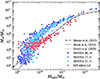 |
Fig. 1. M★–Mhalo relation for isolated galaxies within our simulated Local Group analogues, containing gas and stars and with DM halo masses between 109 M⊙ and 1012.5 M⊙. Galaxies from the HESTIA simulations are coloured in shades of blue, and galaxies from NIVARIA-LG in red. The M★ − Mhalo relations from Moster et al. (2013), Brook et al. (2014), and Girelli et al. (2020) are shown in dotted-dashed, dashed, and dotted lines, respectively. |
3. Results
3.1. Dark galaxies selection sample
We selected samples of dark galaxies and bright galaxies from each simulation at z = 0. Both samples are defined within a sphere of 2.5 Mpc in radius centred on the MW analogues to ensure the search within the highest-resolution regions of the Local Group. We selected only galaxies with a DM halo mass in the [109 − 1010] M⊙ range and a fraction of high-resolution DM particles greater than 0.98. The upper limit of 1010 M⊙ is chosen because we do not expect any galaxy above this halo mass to remain dark, while the lower limit of 109 M⊙ is dictated by the resolution and the necessity of having both dark and bright galaxies within the same halo mass range.
Here, we define dark galaxies as those haloes that, following the conditions described above, have ≤10 stellar particles and ≥10 gas particles. This is ≲105 M⊙ in stellar mass and ≳105 − 106 M⊙ in gas mass, depending on the resolution of the simulations. The number of gas particles was chosen to guarantee that the predicted dark galaxies preserve sufficient gas to remain detectable with radio telescopes. On the other hand, we select a sample of bright galaxies as those haloes that contain more than 10 stellar particles. In this case, we do not restrict ourselves to a minimum number of gas particles. Hence, some of these galaxies could be gas-free at z = 0 (and hence non-star-forming), due to gas exhaustion after SF, ram pressure stripping (Gunn & Gott 1972), or other processes such as interaction with the cosmic web (e.g. Benítez-Llambay et al. 2013).
Table 1 shows the number of galaxies found after applying the selection cuts described above. From the second and third columns we note that, as expected, the total number of galaxies depends on the total mass of the simulation within our designated region, with the most massive simulation containing the largest number of galaxies. However, the number of bright galaxies in the HESTIA simulations is much larger than the number of dark galaxies, whereas the opposite is true for NIVARIA-LG. This difference is likely a consequence of the different SF density thresholds employed in the two simulation sets. Therefore, we do not apply any mass rescaling to the predicted numbers of dark and bright galaxies based on the total Local Group mass, as these numbers depend not only on mass but also on the underlying subgrid physics models of each simulation. Finally, the number of satellites in each sample is indicated in brackets, i.e. haloes belonging to a central or host galaxy. In both HESTIA and NIVARIA-LG, a much higher fraction of bright galaxies are satellites compared to dark galaxies, suggesting that bright galaxies tend to reside closer to other systems and may experience more interactions.
It is important to note that the selection cuts for dark galaxies could be affected by the different particle resolutions of HESTIA and NIVARIA-LG. In Fig. 1, for halo masses below ∼5 × 10⁹ M⊙, HESTIA simulations can form less massive isolated galaxies than NIVARIA-LG. This difference can be attributed to the combination of lower mass resolution and a more restrictive SF criterion adopted in NIVARIA-LG. If NIVARIA-LG had the same particle resolution as HESTIA while preserving its SF density threshold, we would expect a slightly smaller number of dark galaxies. A higher resolution would lower the effective halo mass threshold required for SF, increasing the number of haloes that host stellar particles at a fixed halo mass. In this sense, our predictions should be regarded as an upper limit to the number of dark galaxies expected in the Local Group.
To visualise the distribution of the sample, Fig. 2 shows the number of dark and bright galaxies as a function of DM halo mass, combining all the simulation sets in the left panel, from HESTIA only in the top right panel, and from NIVARIA-LG only in the bottom right panel. The values in brackets in the legends correspond to the total number of galaxies for each case. Bright galaxies dominate the more massive halo region of the plot, whereas dark galaxies are more abundant in the lower-mass end of the distribution. This tendency is consistent with the galaxy sample selection from Lee et al. (2024).
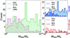 |
Fig. 2. Number of galaxies from the four simulations as a function of the DM halo mass (left panel). The total sample of dark galaxies is shown in magenta and the total sample of bright galaxies is shown in green. The right panels show the same distributions separately for HESTIA simulations in blue (top) and for NIVARIA-LG simulations in red (bottom), representing dark and bright galaxies with dotted-dashed and solid lines, respectively. |
In the top panel of Fig. 3, we show the M★–Mhalo relation for dark and bright galaxies at z = 0 (referred as DGs and BGs in legends hereafter, respectively), in tandem with the semi-empirical relations from Moster et al. (2013), Brook et al. (2014), and Girelli et al. (2020). Similarly, we show the relation between the gas and the halo masses in the central panel, and the relation between the H I gas and the halo masses at the bottom (see Sect. 3.5 for details on how H I is computed in each simulation). Cloud-9 is included in the top and bottom panels for reference, assuming M200 ∼ 5 × 10⁹ M⊙ (Benitez-Llambay & Navarro 2023), an upper stellar mass limit of 105 M⊙ (Zhou et al. 2023; Benítez-Llambay et al. 2024), and MH I ≈ 106 M⊙ (Benítez-Llambay et al. 2024). It falls within the massive end of our dark galaxies region.
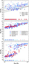 |
Fig. 3. M★–Mhalo relation (top), gas-to-halo mass relation (centre), and H I-to-halo mass relation (bottom), for dark (filled markers) and bright (empty markers) galaxies at z = 0. Galaxies from the HESTIA simulations are coloured in shades of blue and galaxies from NIVARIA-LG are in red. Circles indicate dark galaxies with stars, whereas squares indicate starless dark galaxies. In the top panel, the M★–Mhalo relations from Moster et al. (2013), Brook et al. (2014), and Girelli et al. (2020) are shown in dotted-dashed, dashed, and dotted lines, respectively. We include Cloud-9 as a black diamond in the top and bottom panels. |
In the top panel of the figure, we see a clear separation between dark and bright galaxies in the y-axis, around 105 M⊙ in stellar mass and a large number of starless galaxies, especially for NIVARIA-LG, which we show as squares. More specifically, the number of starless dark galaxies in our sample is 17 for the HESTIA 09_18 run, 11 for HESTIA 17_11, 0 for HESTIA 37_11, and 59 for the NIVARIA-LG simulation (see Table 1). That is, the whole sample of NIVARIA-LG dark galaxies is composed of completely starless objects.
However, in the central panel, the total gas mass exhibits a clear correlation with the DM halo mass, and the dark and bright galaxy samples appear broadly similar in this respect. Some bright galaxies, however, have no gas content and are therefore non-star-forming at the present time. In contrast, in the bottom panel of Fig. 3, the H I gas content differs between the two samples: only the most massive dark galaxies have H I masses comparable to their bright counterparts, i.e. MH I > 105 M⊙ for Mhalo > 109.5 M⊙.
3.2. Dark matter halo properties
In this section, we tackle the evolution of the DM halo mass and its relation to reionisation, as well as intrinsic properties of the haloes, such as the concentration and the spin parameter.
In order to analyse the impact of reionisation, we need to estimate the evolution with time of the minimum critical halo mass needed for gas to collapse and form stars. Following the scheme given in Benitez-Llambay & Frenk (2020), before reionisation the critical DM halo mass corresponds to the one above which atomic hydrogen can cool efficiently to form stars
 (1)
(1)
On the other hand, after the reionisation sets off, the critical DM halo mass for which gas can collapse within haloes is
 (2)
(2)
where Tb refers to the virial temperature of the halo.
In Fig. 4, we show such a critical mass as a function of z. We compare the median halo mass evolution of our dark (dotted-dashed lines) and bright (solid lines) galaxies for HESTIA simulations in blue and NIVARIA-LG in red, together with theoretical predictions. Here, the cyan dashed line represents  for a fixed halo with Tb = 2 × 10⁴ K, and the orange line represents
  . By combining the two relations prior to and after reionisation, Benitez-Llambay & Frenk (2020) show the global critical mass for which the gas can collapse across redshift, represented in Fig. 4 by the black dotted-dashed line, leading to a minimum halo of M200 ∼ 5 × 10⁹ M⊙ at z = 0. Thus, a halo that lies below the black dotted-dashed line should remain completely dark (see also Pereira-Wilson et al. 2023). This plot displays a substantial difference between dark and bright galaxies, where the former tend to lie close to or below the critical mass, whilst the latter are well above the black line at all z, indicating their luminous nature.
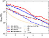 |
Fig. 4. Evolution of the median DM halo masses of dark galaxies (dotted-dashed lines) and bright galaxies (solid lines) as a function of redshift. Red lines represent the median of all galaxies of the NIVARIA-LG simulation, whilst blue lines correspond to the median of all galaxies for the HESTIA runs. The red and blue dots indicate the redshifts at which the galaxies reach half of their final halo mass. Following the scheme from Benitez-Llambay & Frenk (2020), we show with the dotted-dashed grey line the critical mass needed for gas to collapse. In addition, the dashed cyan line shows the critical halo mass for a fixed virial temperature of Tb = 2 × 10⁴ K. The dashed orange line represents the halo mass above which atomic hydrogen cooling is efficient. |
We can observe that dark galaxies generally form later on than bright galaxies, their half-mass accretion time being zdark = 2.0 and zdark = 1.7 for NIVARIA-LG and HESTIA, respectively, while the formation time of the corresponding bright galaxies is between zbright = 3.2 and zbright = 2.6. This result is in agreement with the findings presented in Lee et al. (2024) (their Fig. 5 and discussion therein). In Fig. 4 it is also clear that bright galaxies, which are overall more massive than dark galaxies (see Fig. 2), were already more massive prior to reionisation, making them less vulnerable to the effects of an ionising background. The later formation times of dark galaxies should be reflected in the concentration parameters of their DM haloes, as these systems formed in a less dense Universe.
Figure 5 shows the relation between the halo mass and the concentration corresponding to the DM haloes with an NFW profile at z = 0, where the dashed black line represents the c200 − M200 relation from Dutton & Macciò 2014, following a Planck cosmology. In this figure, the dotted-dashed grey line corresponds to the lineal fit of the data (both dark and bright galaxies), and the shaded region is the 3σ scatter between this fit and the Dutton & Macciò (2014) relation. As expected, we see that the dark galaxy sample has less concentrated DM haloes than bright galaxies at a fixed halo mass. Quantitatively, dark galaxies have a median value of cNFWdark = 11.1 ± 0.5, and bright galaxies a median value of cNFWbright = 18.6 ± 0.5. Cloud-9, also added in the plot, lies close to the Dutton & Macciò (2014) relation.
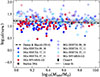 |
Fig. 5. Concentration-halo mass relation for dark (filled markers) and bright (empty markers) galaxies at z = 0, colour-coded as in Fig. 3. The dashed black line is the c200 relation drawn from Dutton & Macciò (2014), and the dotted-dashed grey line represents a lineal fit of both the dark and bright sample together, i.e. log10(cNFW) = − 0.01 log10(Mhalo/M⊙)+1.27. The shaded region shows the 3σ scatter of both relations. |
We then study the spin parameter of the DM haloes in both samples, shown in Fig. 6. The spin parameter, λ, is defined by the following expression (Bullock et al. 2001)
 (3)
(3)
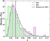 |
Fig. 6. Probability density distribution of the spin parameter of the DM halo, P(λ), for dark galaxies in magenta and bright galaxies in green in all four simulations. The vertical dashed lines indicate the median values for each distribution, being λdark = 0.036 ± 0.003 for dark galaxies, and λbright = 0.026 ± 0.002 for bright galaxies. The solid grey line represents the log-normal fiducial distribution from Bullock et al. (2001), and the dashed grey line indicates its median, i.e. λ0 = 0.035 ± 0.005. |
where J is the angular momentum of a sphere with mass M and radius R, and V is the circular velocity at R.
We compare the resulting distributions of the spin parameters with the log-normal distribution from Bullock et al. (2001) as a reference. Dark galaxies (coloured magenta) show larger spin parameters than bright galaxies (coloured green), with median values of λdark = 0.036 ± 0.003 and λbright = 0.026 ± 0.002, respectively. The significance in the difference between both distributions is confirmed by applying the Kolmogorov-Smirnov (KS) test, which results in a p-value of ∼10−5. Interestingly, the spin-parameter distribution of dark galaxies matches the Bullock et al. (2001) model more closely than that of bright galaxies. This likely reflects the fact that these haloes have experienced little baryonic processing, preserving the ‘pristine’ angular momentum distribution predicted by N-body simulations, whereas SF and feedback in bright galaxies can alter the spin of their host haloes. The larger spin parameters of dark galaxies are directly related to their lower concentrations and may hinder the retention and condensation of gas to form stars, leading to lower gas densities as well (see also Jimenez & Heavens 2020 and Lee et al. 2024).
3.3. Gas content and thermodynamic properties
We study the temperature and density of the gas in both dark and bright galaxies. The relation between these two properties at z = 0 is shown in Fig. 7 as a 2D histogram of gas particles aggregated over all galaxies in each sample. The top row corresponds to dark galaxies, while the bottom row shows bright galaxies. Each column corresponds to a different simulation, from left to right HESTIA 09_18, 17_11, 37_11, and NIVARIA-LG. Regardless of the particular simulation, dark galaxies do not exhibit characteristic star-forming regions in the T–ρ phase diagram, as they lack gas at densities above the threshold required for SF, indicated by the vertical cyan and white line, for HESTIA and NIVARIA-LG, respectively. Bright galaxies contain on average a significant amount of dense gas, while dark galaxies have little to no gas at densities larger than nth.
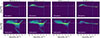 |
Fig. 7. Temperature-density diagram for gas particles in all dark (top row) and all bright (bottom row) galaxies. Each column corresponds to a different simulation, from left to right HESTIA 09_18, 17_11, 37_11, and NIVARIA-LG. The horizontal dashed line indicates the threshold temperature below which gas is able to form stars in NIVARIA-LG, whilst the vertical cyan and white lines show the corresponding density thresholds to set off SF in HESTIA (nth = 0.13 cm−3) and NIVARIA-LG (nth = 10 cm−3), respectively. The continuous red line in the T − ρ diagrams of dark galaxies corresponds to the predicted temperature-density relation expected in RELHICs, as derived in Benítez-Llambay et al. (2017). Note that the dark galaxy histogram corresponding to HESTIA 37_11 is rather sparse, as only one object of this type is found in that simulation. |
In HESTIA simulations, bright galaxies display a region of dense gas in the upper-right part of the plots, owing to the implementation of an effective equation of state (EOS) that imposes an artificial pressure for gas above the SF density threshold (Grand et al. 2017, following the Springel & Hernquist 2003 model). This feature is instead absent in NIVARIA-LG, where the gas is treated as an ideal gas at all densities and a polytropic effective EOS for star-forming gas is not imposed (e.g. Stinson et al. 2012; Wang et al. 2015). In NIVARIA-LG, the more restrictive SF criterion (nth ≥ 10 cm−3) makes it more difficult for galaxies to convert their gas into stars: as a consequence, a given dark galaxy might be able to form some stars in HESTIA, but not in NIVARIA-LG. It should be noted that the absence of gas particles above the SF density threshold in the T–ρ diagram for NIVARIA-LG bright galaxies simply indicates that these systems are not currently forming stars at z = 0. However, they did experience SF at earlier epochs, in contrast to bright galaxies in HESTIA, which are predominantly star-forming at z = 04.
As demonstrated in Benítez-Llambay et al. (2017), gas within dark galaxies should exhibit a characteristic temperature–density relation arising from the combined effects of gas cooling at high densities and photoheating at low densities. This relation has a peak at T ∼ 4 × 10⁴ K and ρ ∼ 10−4.8 cm−3. This prediction, shown in the dark galaxies top panels of Fig. 7 as a solid red line, is in very good agreement with the results from our simulations. This relation reflects an approximate hydrostatic equilibrium between the gas and the halo gravitational potential, as well as thermal equilibrium with the UV background under the assumption of spherical symmetry. The gas properties of dark galaxies thus establish the conditions for little to no SF and are consistent with the characteristics of their underlying DM haloes. Lower halo concentrations, lower halo masses at the epoch of reionisation, and higher spin parameters compared to bright galaxies of similar mass promote under-dense gas to remain in hydrostatic and thermal equilibrium within its DM matter halo and to never form stars.
3.4. Spatial distribution and environment
In order to assess the impact of the intergalactic medium on the properties of dark galaxies, in this section we analyse whether dark and bright galaxies inhabit different environments and how the density of these surroundings evolves over time. Figure 8 shows the distribution of dark (magenta) and bright (green) galaxies in both the x − y and x − z projections for the four simulation runs at the present epoch. The figure displays a region centred on the MW analogue and extending to a radius of 2.5 Mpc. The background represents the superimposed DM and gas density fields. Bright galaxies are generally more concentrated in high-density regions, closer to the two main central galaxies. In contrast, the distribution of dark galaxies appears to be more spatially extended, occupying larger radial distances, and residing predominantly farther from the central regions and the bulk of the main filament. This trend is less evident in NIVARIA-LG, because the sample of bright galaxies is significantly smaller than that of dark galaxies; nevertheless, the trend is still present.
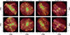 |
Fig. 8. Projected positions of dark (magenta) and bright (green) galaxies in the x − y (top row) and x − z (bottom row) planes at z = 0, within a sphere of 2.5 Mpc of radius from the MW. From the left to right, we present the three HESTIA simulations (09_18, 17_11, and 37_11) and NIVARIA-LG. Circles indicate dark galaxies with stars, whereas squares indicate the starless dark galaxies. The background shows the density of DM in orange and the gas density in yellow. The region is centred on the MW, shown as a blue triangle, while M31 is represented as a blue cross mark. |
The larger distances from the MW at which dark galaxies are found are further illustrated in Fig. 9, which shows the cumulative distribution of the radial distances of all dark (magenta) and bright (green) galaxies from the MW analogues. The difference between the two radial distributions is again confirmed by a KS test, yielding a p-value of ∼10−10. This low value indicates that the two samples are statistically distinct. We find that 50% of the dark galaxy sample lies within 1.9 Mpc of the MW, whereas 50% of bright galaxies are located within 1.3 Mpc. Consequently, we expect a large fraction of dark galaxies to be found on the outskirts of the Local Group.
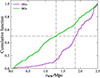 |
Fig. 9. Cumulative distribution of the radial distances of dark (magenta) and bright (green) galaxies with respect to the MW analogues for all four simulations at z = 0. The horizontal grey line marks the mean of the distributions, while the two vertical lines indicate the distances within which 50% of dark and bright galaxies are found, corresponding to rMW = 1.9 Mpc and rMW = 1.3 Mpc, respectively. |
We take a step further and examine the evolution of the DM and gas densities within a spherical shell extending from 1 Rvir to 7 Rvir around each dark and bright galaxy identified at different redshifts. The results are shown in Fig. 10, where the median densities of all dark and bright galaxies from the four simulations are displayed in magenta and green, respectively. The shaded background regions represent the 16th and 84th percentiles of each distribution. Consistent with the results shown in Fig. 8, bright galaxies reside in environments with higher DM and gas densities than dark galaxies. These results indicate that dark galaxies originate in lower-density regions within the Local Group and remain in such environments throughout their lifetime. Their persistently lower DM and gas density environment make dark galaxies less susceptible to galaxy interactions, mergers, and gas inflows, allowing their gas to remain diffuse and in equilibrium within their DM halo rather than collapsing. These results are in agreement with previous work by Benítez-Llambay et al. (2017), who showed that gas-rich RELHICs inhabit the under-dense outskirts of the APOSTLE simulations. In Appendix A, we present the same density evolution as shown in Fig. 10, but separately for each simulation. We also include the evolution of the median Rvir of all dark and bright galaxies in the upper panels of Fig. A.1, as a reference to the physical scales involved with respect to the defined environment.
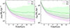 |
Fig. 10. Evolution of median DM (left panel) and gas (right panel) density of the environment around the full sample of dark galaxies in magenta and bright galaxies in green, combining all four simulations. The shaded backgrounds are the regions limited by the 16th and 84th percentiles of the distributions. The environment is defined as a spherical shell between 1 Rvir and 7 Rvir of each halo, at each redshift. |
3.5. H I detectability with FAST
Objects such as dark galaxies, which exhibit little to no luminous matter, are inherently difficult to identify observationally. Nevertheless, if they contain a substantial reservoir of H I they may be detectable as gas clouds via their 21 cm line emission, using facilities such as the FAST radio telescope. In this section, we present estimates of the detectability of dark galaxies based on their H I content, selecting FAST as the instrument of choice due to its large sky coverage and high sensitivity.
We estimate the amount of neutral atomic hydrogen in the HESTIA sample by adopting the empirical approach presented in Arjona-Gálvez et al. (2024). This method builds on the phenomenological prescription introduced by Marinacci et al. (2017), itself based on Leroy et al. (2008). In this framework, the ratio between the densities of molecular and atomic hydrogen columns is fitted with a functional form that depends on the gas mid-plane pressure, which then allows us to infer the H I atomic fraction. On the other hand, the H I fraction in NIVARIA-LG is measured following the self-shielding approximation detailed in Rahmati et al. (2013), which uses the radiative transfer model from Pawlik & Schaye (2008, 2011).
Figure 11 shows the H I masses of the dark galaxy sample in the HESTIA simulations (blue shades) and NIVARIA-LG (red), as a function of their DM halo masses. We include Cloud-9 as a reference5. We can observe a very strong correlation between the halo mass and the H I gas in each dark galaxy. We performed an exercise to furnish a quick estimate on the detectability of these dark galaxies with FAST. Details on how the FAST limits are calculated can be found in Appendix B. The two shaded areas in Fig. 11 represent the detectability region within 1 Mpc and 2.5 Mpc, according to the values obtained for the minimum H I mass detectable with FAST. Here, it can be seen that up to 18 of our dark galaxies fall in the region corresponding to distances within 1 Mpc, and up to ten of those fall in the region within 2.5 Mpc. These maximum values are set by the NIVARIA-LG simulation, which contributes the largest number of dark galaxies within the detectability region compared to the rest of the simulations. It is also clear that several dark galaxies are below the detection limits for such distances.
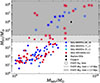 |
Fig. 11. Mass of H I versus DM halo mass for dark galaxies in each simulation, with HESTIA indicated as blue shades, while NIVARIA-LG is shown in red. Squares denote starless dark galaxies. The grey shaded regions represent galaxies with H I masses that could be detectable with FAST in 1 hour of integration time and at distances of < 1 Mpc and < 2.5 Mpc from the MW analogues. The concentric circles indicate dark galaxies whose central H I column densities exceed the FAST detection limit, NH I. We include Cloud-9 as a black diamond. |
In Fig. 12 we further clarify the distance dependence by showing the H I masses of dark galaxies with respect to their distance from the simulated MW analogues. The dotted-dashed grey line represents the H I mass limit with respect to the distance, as given by Eq. B.3. All dark galaxies located above this line should be detectable by FAST in terms of their total H I mass and distance. The area of detectability is shown as the grey shaded region. In this case, the number of dark galaxies falling within this region is between 0 and 18, according to each of the simulation runs used (where NIVARIA-LG provides the largest estimate and HESTIA 37_11 the lowest).
 |
Fig. 12. H I mass versus radial distance of dark galaxies with respect to the MW analogues in each simulated run, with HESTIA indicated as blue shaded symbols and NIVARIA-LG as red symbols. Squares correspond to starless dark galaxies. The dotted-dashed grey line represents the minimum H I mass that galaxies must have to be detectable by FAST, as a function of their distance from us. Dark galaxies likely to be detectable by FAST are those that fall within the shaded region. The concentric circles indicate dark galaxies whose central H I column densities NH I exceed the FAST detection limit. Cloud-9 is included as a black diamond at d = 4.7 Mpc. |
We further explore the detectability of these galaxies by analysing their H I column density profiles, which are shown in Fig. 13, for HESTIA in the left panel and for NIVARIA-LG in the right panel. The profiles are coloured according to the H I mass of each dark galaxy, where darker colours indicate larger H I masses. The coloured vertical dotted-dashed lines indicate the softening length of each simulation, below which profiles are not well resolved. Since FAST can reach a median 3σ column density of NH I = 2 × 1017 cm−2 (Pan et al. 2024), we show this limit in the panels as a horizontal dotted-dashed grey line. Hence, all galaxies whose profiles lie above this threshold and within the grey shaded area would be detectable by FAST. We can see that all profiles with values that exceed the FAST column density detection limit (and beyond the softening length) have H I masses > 104 M⊙. These results are added to Fig. 11 and Fig. 12, where we now indicate the galaxies corresponding to these minimum detectable column densities using concentric circles. Therefore, there is a trend in which the most massive dark galaxies in DM are generally those that can be detectable, in agreement with results from Benítez-Llambay et al. (2017). On the other hand, since the simulated dark galaxies have been centred and set in a face-on orientation, the NH I values shown in Fig. 13 are actually a lower limit and could be slightly larger when placing the galaxies edge-on.
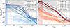 |
Fig. 13. H I column density profiles of dark galaxies for the HESTIA simulations (left) and the NIVARIA-LG simulations (right), coloured by H I mass. The dotted-dashed grey line represents the minimum H I column density value that FAST can reach, which is NH I = 2 × 1017 cm−2. The coloured shaded area in each panel shows the softening length corresponding to each simulation. A smaller number of dark galaxies could be detected by the less sensitive ALFALFA Survey, whose sensitivity is NH I ≳ 2 × 1018 cm−2. |
However, the total number of dark galaxies with both sufficient H I mass and column densities to be detectable by FAST is up to 14 when using the NIVARIA-LG simulation, which therefore provides an upper limit: these galaxies are indicated as red symbols with concentric circles within the shaded grey region in Fig. 12. Conversely, only five and seven dark galaxies would be detectable by FAST, according to the HESTIA simulations (seeds 09_18 and 17_11). Since the simulations consider the whole sky, these values are effectively smaller when we account for the fact that FAST is located in the northern hemisphere and covers only ∼58% of the total sky (e.g. Qian et al. 2020).
Consequently, the upper limit on the number of dark galaxies detectable within 2.5 Mpc from the MW, taking into account the FAST sky coverage and minimum H I mass and column density, is eight. This is our preferred value, based on the more realistic NIVARIA-LG simulations, which, notably, produce all starless dark galaxies.
4. Discussion
We find that bright galaxies in our sample include a substantially higher fraction of satellites than dark galaxies, indicating that luminous systems are more frequently bound to larger hosts, while dark galaxies preferentially reside in isolation. This environmental distinction also appears in the satellite statistics of Lee et al. (2024), where star-rich galaxies exhibit higher satellite fractions than star-poor or starless systems. In our simulations, these differences naturally place bright and dark galaxies in contrasting environments: bright galaxies experience more mergers, interactions, and tidal capture, whereas dark galaxies remain largely detached from dense environments and massive hosts. This is fully consistent with the environmental-density trends presented in Sect. 3.4, which show that dark galaxies lie farther from the main filaments and central regions of the Local Group. Moreover, as shown in Fig. 10, not only do dark galaxies inhabit lower-density regions today, but they also originate in under-dense environments, which can directly suppress SF by limiting gas accretion. Although at very high redshift this scenario holds uncertainties due to the much higher and uniform global density of the Universe and the limitations of the simulations, the median trends in Fig. 10 still show a difference of the order of ∼0.1 dex in both DM and gas density at early epochs. This picture is also supported by observational results from Kwon et al. (2025), who find that potential dark galaxy candidates in the ALFALFA survey preferentially occupy low-density environments.
The distinct formation histories of bright and dark galaxies further reinforce this scenario. As shown in Fig. 4, dark galaxies assemble later (zdark = 1.7 − 2.0) than bright galaxies (zbright = 2.6 − 3.2), resulting in systematically lower concentrations (Fig. 5). Combined with their higher spin parameters, this implies that dark galaxies inhabit more extended, less concentrated haloes that retain under-dense gas, below the SF threshold.
These findings are in excellent agreement with results from Benítez-Llambay et al. (2017) and Lee et al. (2024), even though their studies employed a different simulation suite, numerical methods, resolution, and initial conditions. An important difference from the work of Lee et al. (2024), however, is that they do not require their sample of dark galaxies to necessarily contain H I gas, while in our selection we explicitly require H I gas to be present, in order to assess the detectability of dark galaxies with observational surveys. The comparison with Lee et al. (2024) should therefore be considered qualitative, since the dark galaxy samples in our work and theirs are selected using different underlying criteria.
In a recently submitted work, Zheng et al. (2025) studied a sample of dark galaxies in the HESTIA and AURIGA simulations, focusing on faint systems with Mg > −10 and MH I > 105 M⊙. In their sample, only one completely starless object is identified, found in AURIGA. As shown in our Fig. 11, we also do not find any starless dark galaxies in HESTIA with MH I > 105 M⊙, although such objects do appear in NIVARIA-LG, which we attribute to the more restrictive SF conditions adopted in this simulation. Despite the different selection criteria, our results are broadly consistent with those of Zheng et al. (2025). Their study primarily examines simulations that employ similar subgrid physics (HESTIA and AURIGA), whereas we compare dark and luminous galaxies across two Local Group simulations that adopt different physical models and SF prescriptions, allowing us to assess the robustness of dark galaxy predictions across distinct simulation setups. Zheng et al. (2025) also provide predictions for the number density of dark galaxies within a given volume. However, differences in selection criteria make direct comparisons non-trivial.
5. Conclusions
In this work, we analysed the three high-resolution HESTIA simulation runs (Libeskind et al. 2020) and the new NIVARIA-LG simulation (Contreras-Santos et al., in prep.) to derive the properties of H I-rich dark galaxies within Local Group–like volumes simulated with the same constrained initial conditions but with different numerical codes and galaxy-formation models (AREPO for the HESTIA simulation, GASOLINE2 for NIVARIA-LG). Across the four runs, we identified a total of 114 dark galaxies in the DM halo mass range 109 − 1010 M⊙, of which only six are satellites of larger galactic systems at z = 0. We then compared their properties with those of a control sample of bright galaxies within the same halo mass range. Our main conclusions are summarised below.
Dark galaxies:
-
exist in Local Group simulations run with different codes and feedback models, with their abundance depending on the mass of the Local Group itself and, critically, on the adopted SF density threshold nth. Simulations that employ a more realistic, higher nth, produce significantly more dark galaxies than those that do not (up to ∼60 in the NIVARIA-LG run, compared to 17, 11, and 0 starless dark galaxies arising, respectively, in the three HESTIA runs, as shown in Table 1);
-
contain a similar total amount of gas as their bright-galaxy counterparts, although only the most massive dark galaxies, with Mhalo > 109.5 M⊙, have large H I gas reservoirs comparable to those found in bright galaxies, i.e. MH I > 105 M⊙ (Fig. 3). Such a gas cannot form stars efficiently because of its low density, being in hydrostatic equilibrium within the gravitational potential of its halo (Fig. 7);
-
have lower masses than bright galaxies at the epoch of reionisation, and throughout cosmic time (Fig. 4), which render them dark, since galaxy formation can occur only in haloes whose masses exceed a critical threshold (Benitez-Llambay & Frenk 2020);
-
have z = 0 halo masses peaking at ∼2 × 10⁹ M⊙ (Fig. 2), higher spin parameters (Fig. 6), and lower concentrations (Fig. 5) than bright galaxies, consistent with their late formation times (Fig. 4);
-
are located farther from the MW than luminous galaxies (Fig. 9), with about 80% residing at distances greater than 1.5 Mpc, and inhabit lower-density regions of the Local Group (Fig. 8);
-
formed and evolved across redshift within regions characterised by persistently lower DM and gas densities compared to the environments of bright galaxies, making them less susceptible to galaxy interactions, mergers, and gas inflows (Fig. 10);
-
can be detected via their H I emission. Using the sky coverage of the new FAST radio telescope, along with its minimum detectable H I mass and column-density sensitivity, we predict that up to eight dark galaxies should be detectable in H I within 2.5 Mpc of the Local Group (Figs. 11 and 12).
The NIVARIA-LG simulation adopts an SF density threshold, nth = 10 cm−3, which is more realistic than the HESTIA simulation, reflecting the densities of clumps within typical giant molecular clouds (10 − 100 cm−3). It produces a great match of the M★–Mhalo relation over several orders of magnitude in halo mass (Fig. 1) and is the only simulation able to generate completely starless dark galaxies with substantial H I masses, MH I > 104−5 M⊙, (Fig. 11 and Fig. 12). Thanks to its physically motivated SF recipe, NIVARIA-LG is likely to provide the most reliable predictions for dark galaxies with sufficient H I to be detectable. Indeed, while all dark galaxies remain completely starless in NIVARIA-LG, the low SF density threshold adopted in HESTIA allows some dark galaxies to form a small number of stars.
The study of dark galaxies is currently a highly active field of research, driven by the increasing availability of both observational data and theoretical predictions. Improvements in observational techniques are expanding the number of dark galaxy candidates, while advances in numerical simulations, now able to reproduce many of the key processes governing galaxy formation and evolution, are proving essential for interpreting these systems. Together, these developments are pushing the field forward and bringing us closer to a robust confirmation of genuine dark galaxies. Such objects would serve as powerful cosmological probes of the ΛCDM model, and their detection would provide strong support for it. We expect upcoming observations with FAST, along with other radio telescopes, to aid in the detection of H I sources harboured within a DM halo. Future work should focus on measuring the gas metallicity within dark galaxies, to determine whether truly starless systems indeed contain primordial, metal-free gas, and to assess whether any past SF episodes may have occurred.
Acknowledgments
We thank Julio Navarro, Duncan Forbes, Jonah Gannon and Marco Monaci for useful discussions. We thank the anonymous referee for the helpful comments and suggestions for this work. ADC, GGB, and ACS acknowledge financial support from the Spanish Ministry of Science and Innovation (MICINN), Consolidación Investigadora program, CNS2023-144669, project “Tiny” (PI A. Di Cintio), and the 2024 call “Proyectos de Generación de Conocimiento”, grant number PID2024-160009NA-I00, proyecto “INGENIO”. SC acknowledges funding from the State Research Agency (AEI-MICINN) under the grant with reference PID2023-149139NB-I00. EAG acknowledges support from (AEI-MICINN) and the European Social Fund (ESF+) through a FPI grant PRE2020-096361. SCB acknowledges financial support from the (MICINN) through RYC2022-035838-I, PID2021-128131NB-I00 (CoBEARD) and CNS2022-135482 projects. AN is supported by the applied research and innovation project (SOL2024-31834, PI Andrea Negri), co-financed by the EU - Ministry of Finance and Public Service – European Funds – Junta de Andalucía – Consejería de Universidad, Investigación e Innovación. AK is supported by project PID2024-156100NB-C21 financed by MICIU /AEI/10.13039/501100011033/FEDER, UE and further thanks Fontaines DC for hurricane laughter. This research is also co-funded by the European Union (Widening Participation, ExGal-Twin, GA 101158446 “UNDARK”, GA 101159929). The NIVARIA-LG simulations have been run using LaPalma supercomputer, project can43 (PI A. Di Cintio). The authors acknowledge the contribution of the IAC High-Performance Computing support team.
References
- Anand, G. S., Benítez-Llambay, A., Beaton, R., et al. 2025, ApJ, 993, L55 [Google Scholar]
- Arjona-Gálvez, E., Di Cintio, A., & Grand, R. J. J. 2024, A&A, 690, A286 [NASA ADS] [CrossRef] [EDP Sciences] [Google Scholar]
- Arjona-Gálvez, E., Cardona-Barrero, S., Grand, R. J. J., et al. 2025, A&A, 699, A301 [NASA ADS] [CrossRef] [EDP Sciences] [Google Scholar]
- Arora, N., Macciò, A. V., Courteau, S., et al. 2022, MNRAS, 512, 6134 [Google Scholar]
- Benitez-Llambay, A., & Frenk, C. 2020, MNRAS, 498, 4887 [CrossRef] [Google Scholar]
- Benitez-Llambay, A., & Navarro, J. F. 2023, ApJ, 956, 1 [Google Scholar]
- Benítez-Llambay, A., Navarro, J. F., Abadi, M. G., et al. 2013, ApJ, 763, L41 [Google Scholar]
- Benítez-Llambay, A., Navarro, J. F., Frenk, C. S., et al. 2017, MNRAS, 465, 3913 [Google Scholar]
- Benítez-Llambay, A., Dutta, R., Fumagalli, M., & Navarro, J. F. 2024, ApJ, 973, 61 [Google Scholar]
- Blank, M., Macciò, A. V., Dutton, A. A., & Obreja, A. 2019, MNRAS, 487, 5476 [NASA ADS] [CrossRef] [Google Scholar]
- Brook, C. B., Stinson, G., Gibson, B. K., Wadsley, J., & Quinn, T. 2012, MNRAS, 424, 1275 [CrossRef] [Google Scholar]
- Brook, C. B., Di Cintio, A., Knebe, A., et al. 2014, ApJ, 784, L14 [NASA ADS] [CrossRef] [Google Scholar]
- Bullock, J. S., Dekel, A., Kolatt, T. S., et al. 2001, ApJ, 555, 240 [NASA ADS] [CrossRef] [Google Scholar]
- Carlesi, E., Sorce, J. G., Hoffman, Y., et al. 2016, MNRAS, 458, 900 [NASA ADS] [CrossRef] [Google Scholar]
- Chabrier, G. 2003, PASP, 115, 763 [Google Scholar]
- Duffy, A. R., Battye, R. A., Davies, R. D., Moss, A., & Wilkinson, P. N. 2008, MNRAS, 383, 150 [Google Scholar]
- Dutton, A. A., & Macciò, A. V. 2014, MNRAS, 441, 3359 [Google Scholar]
- Dutton, A. A., Obreja, A., Wang, L., et al. 2017, MNRAS, 467, 4937 [Google Scholar]
- Fattahi, A., Navarro, J. F., Sawala, T., et al. 2016, MNRAS, 457, 844 [NASA ADS] [CrossRef] [Google Scholar]
- Ferland, G. J., Korista, K. T., Verner, D. A., et al. 1998, PASP, 110, 761 [Google Scholar]
- Gill, S. P. D., Knebe, A., & Gibson, B. K. 2004, MNRAS, 351, 399 [Google Scholar]
- Giovanelli, R., Haynes, M. P., Kent, B. R., et al. 2005, AJ, 130, 2598 [Google Scholar]
- Girelli, G., Pozzetti, L., Bolzonella, M., et al. 2020, A&A, 634, A135 [NASA ADS] [CrossRef] [EDP Sciences] [Google Scholar]
- Gottloeber, S., Hoffman, Y., & Yepes, G. 2010, ArXiv e-prints [arXiv:1005.2687] [Google Scholar]
- Grand, R. J. J., Gómez, F. A., Marinacci, F., et al. 2017, MNRAS, 467, 179 [NASA ADS] [Google Scholar]
- Gunn, J. E., & Gott, J. R., III 1972, ApJ, 176, 1 [Google Scholar]
- Haardt, F., & Madau, P. 1996, ApJ, 461, 20 [Google Scholar]
- Haynes, M. P., Giovanelli, R., Martin, A. M., et al. 2011, AJ, 142, 170 [Google Scholar]
- Haynes, M. P., Giovanelli, R., Kent, B. R., et al. 2018, ApJ, 861, 49 [Google Scholar]
- Hoeft, M., Yepes, G., Gottlöber, S., & Springel, V. 2006, MNRAS, 371, 401 [NASA ADS] [CrossRef] [Google Scholar]
- Hoffman, Y., & Ribak, E. 1991, ApJ, 380, L5 [NASA ADS] [CrossRef] [Google Scholar]
- Ikeuchi, S. 1986, Ap&SS, 118, 509 [Google Scholar]
- Jimenez, R., & Heavens, A. F. 2020, MNRAS, 498, L93 [Google Scholar]
- Karunakaran, A., & Spekkens, K. 2024, RNAAS, 8, 24 [Google Scholar]
- Kennicutt, R. C., Jr 1998, ApJ, 498, 541 [Google Scholar]
- Kent, B. R., Giovanelli, R., Haynes, M. P., et al. 2007, ApJ, 665, L15 [NASA ADS] [CrossRef] [Google Scholar]
- Knollmann, S. R., & Knebe, A. 2009, ApJS, 182, 608 [Google Scholar]
- Kwon, M., Hwang, H. S., Kent, B. R., et al. 2025, ApJS, 279, 38 [Google Scholar]
- Lee, G., Hwang, H. S., Lee, J., Shin, J., & Song, H. 2024, ApJ, 962, 129 [Google Scholar]
- Leisman, L., Rhode, K. L., Ball, C., et al. 2021, AJ, 162, 274 [NASA ADS] [CrossRef] [Google Scholar]
- Leroy, A. K., Walter, F., Brinks, E., et al. 2008, AJ, 136, 2782 [Google Scholar]
- Li, J., Wang, Y.-G., Kong, M.-Z., et al. 2018, RAA, 18, 003 [Google Scholar]
- Li, D., Stringer, A., Brown, P. E., Eadie, G. M., & Abraham, R. G. 2025a, AnApS, 19, 261 [Google Scholar]
- Li, D. D., Liu, Q., Eadie, G. M., et al. 2025b, ApJ, 986, L18 [Google Scholar]
- Libeskind, N. I., Yepes, G., Knebe, A., et al. 2010, MNRAS, 401, 1889 [CrossRef] [Google Scholar]
- Libeskind, N. I., Carlesi, E., Grand, R. J. J., et al. 2020, MNRAS, 498, 2968 [NASA ADS] [CrossRef] [Google Scholar]
- Liu, X.-L., Xu, J.-L., Jiang, P., et al. 2025, Sci. Adv., 11, eads4057 [Google Scholar]
- Macciò, A. V., Udrescu, S. M., Dutton, A. A., et al. 2016, MNRAS, 463, L69 [CrossRef] [Google Scholar]
- Marinacci, F., Grand, R. J. J., Pakmor, R., et al. 2017, MNRAS, 466, 3859 [Google Scholar]
- Martínez-Delgado, D., Roca-Fàbrega, S., Miró-Carretero, J., et al. 2023, A&A, 669, A103 [NASA ADS] [CrossRef] [EDP Sciences] [Google Scholar]
- Meyer, M., Robotham, A., Obreschkow, D., et al. 2017, PASA, 34, 52 [Google Scholar]
- Minchin, R., Davies, J., Disney, M., et al. 2005, ApJ, 622, L21 [NASA ADS] [CrossRef] [Google Scholar]
- Moster, B. P., Naab, T., & White, S. D. M. 2013, MNRAS, 428, 3121 [Google Scholar]
- Navarro, J. F., Frenk, C. S., & White, S. D. M. 1996, ApJ, 462, 563 [Google Scholar]
- Navarro, J. F., Frenk, C. S., & White, S. D. M. 1997, ApJ, 490, 493 [Google Scholar]
- Nebrin, O., Giri, S. K., & Mellema, G. 2023, MNRAS, 524, 2290 [Google Scholar]
- Nelson, D., Pillepich, A., Springel, V., et al. 2019, MNRAS, 490, 3234 [Google Scholar]
- Okamoto, T., Gao, L., & Theuns, T. 2008, MNRAS, 390, 920 [Google Scholar]
- Pakmor, R., Springel, V., Bauer, A., et al. 2016, MNRAS, 455, 1134 [Google Scholar]
- Pan, H., Jarvis, M. J., Zhu, M., et al. 2024, MNRAS, 534, 202 [Google Scholar]
- Pawlik, A. H., & Schaye, J. 2008, MNRAS, 389, 651 [NASA ADS] [CrossRef] [Google Scholar]
- Pawlik, A. H., & Schaye, J. 2011, MNRAS, 412, 1943 [Google Scholar]
- Pereira-Wilson, M., Navarro, J. F., Benítez-Llambay, A., & Santos-Santos, I. 2023, MNRAS, 519, 1425 [Google Scholar]
- Pillepich, A., Nelson, D., Springel, V., et al. 2019, MNRAS, 490, 3196 [Google Scholar]
- Planck Collaboration XVI. 2014, A&A, 571, A16 [NASA ADS] [CrossRef] [EDP Sciences] [Google Scholar]
- Pontzen, A., Roškar, R., Stinson, G., & Woods, R. 2013, Astrophysics Source Code Library[record ascl:1305.002] [Google Scholar]
- Qian, L., Yao, R., Sun, J., et al. 2020, The Innovation, 1, 100053 [NASA ADS] [CrossRef] [Google Scholar]
- Rahmati, A., Pawlik, A. H., Raičević, M., & Schaye, J. 2013, MNRAS, 430, 2427 [NASA ADS] [CrossRef] [Google Scholar]
- Read, J. I., Iorio, G., Agertz, O., & Fraternali, F. 2017, MNRAS, 467, 2019 [NASA ADS] [Google Scholar]
- Rees, M. J. 1986, MNRAS, 218, 25P [Google Scholar]
- Roberts, M. S. 1975, in Galaxies and the Universe, eds. A. Sandage, M. Sandage, & J. Kristian, 309 [Google Scholar]
- Santos-Santos, I. M., Di Cintio, A., Brook, C. B., et al. 2018, MNRAS, 473, 4392 [NASA ADS] [CrossRef] [Google Scholar]
- Sawala, T., Frenk, C. S., Fattahi, A., et al. 2016, MNRAS, 457, 1931 [Google Scholar]
- Schmidt, M. 1959, ApJ, 129, 243 [NASA ADS] [CrossRef] [Google Scholar]
- Shen, S., Wadsley, J., & Stinson, G. 2010, MNRAS, 407, 1581 [NASA ADS] [CrossRef] [Google Scholar]
- Sorce, J. G., Gottlöber, S., Yepes, G., et al. 2016, MNRAS, 455, 2078 [NASA ADS] [CrossRef] [Google Scholar]
- Springel, V. 2010, MNRAS, 401, 791 [Google Scholar]
- Springel, V., & Hernquist, L. 2003, MNRAS, 339, 289 [Google Scholar]
- Stinson, G. S., Brook, C., Macciò, A. V., et al. 2012, MNRAS, 428, 129 [Google Scholar]
- Trentham, N., Möller, O., & Ramirez-Ruiz, E. 2001, MNRAS, 322, 658 [Google Scholar]
- Tully, R. B., Courtois, H. M., Dolphin, A. E., et al. 2013, AJ, 146, 86 [NASA ADS] [CrossRef] [Google Scholar]
- van Loon, J. T., Stanimirović, S., Putman, M. E., et al. 2009, MNRAS, 396, 1096 [Google Scholar]
- Vogelsberger, M., Genel, S., Sijacki, D., et al. 2013, MNRAS, 436, 3031 [Google Scholar]
- Wadsley, J. W., Keller, B. W., & Quinn, T. R. 2017, MNRAS, 471, 2357 [NASA ADS] [CrossRef] [Google Scholar]
- Wang, L., Dutton, A. A., Stinson, G. S., et al. 2015, MNRAS, 454, 83 [NASA ADS] [CrossRef] [Google Scholar]
- Waterval, S., Macciò, A. V., Buck, T., et al. 2024, MNRAS, 533, 1463 [CrossRef] [Google Scholar]
- Weinberger, R., Springel, V., & Pakmor, R. 2020, ApJS, 248, 32 [Google Scholar]
- White, S. D. M., & Rees, M. J. 1978, MNRAS, 183, 341 [Google Scholar]
- Xu, J.-L., Zhu, M., Yu, N., et al. 2023, ApJ, 944, L40 [NASA ADS] [CrossRef] [Google Scholar]
- Zaroubi, S., Hoffman, Y., & Dekel, A. 1999, ApJ, 520, 413 [NASA ADS] [CrossRef] [Google Scholar]
- Zhang, C.-P., Zhu, M., Jiang, P., et al. 2024, Sci. Chin. Phys. Mech. Astron., 67, 219511 [CrossRef] [Google Scholar]
- Zheng, H., Jiang, F., Liao, S., & Libeskind, N. I. 2025, ArXiv e-prints [arXiv:2511.16726] [Google Scholar]
- Zhou, R., Zhu, M., Yang, Y., et al. 2023, ApJ, 952, 130 [CrossRef] [Google Scholar]
We note that, in the current NIVARIA-LG sample, all bright galaxies appear quenched at z = 0. This may reflect environmental effects within the Local Group volume (e.g. cosmic-web stripping or backsplash objects), and will be explored in future higher-resolution NIVARIA-LG simulations.
Note that here Cloud-9 is not within the range of distances of our analysis, i.e. dCloud − 9 ∼ 4.7 Mpc.
Appendix A: Evolution of the density of the environment
We present in Fig. A.1 the median densities of the environment around dark and bright galaxies for each simulation individually. In this figure, dark galaxies are represented as dotted-dashed lines and bright galaxies as solid lines. Here, the peaks are owing to pericentric passages of galaxies that become satellites of other galaxies at different times, and therefore the density of their environment rises steeply because of the presence of a larger galaxy. Note that the dotted-dashed cyan line refers to the only dark galaxy found in the HESTIA run 37_11, which is currently a satellite galaxy (see Table 1).
Appendix B: FAST detection limits
We follow the procedure presented in Li et al. (2018), done to obtain the integration time and number of detectable galaxies.
Firstly, we need the thermal noise associated to the instrument (Duffy et al. 2008)
 (B.1)
(B.1)
where k = 1380 Jy m2 K−1 is the Boltzmann constant, Tsys is the temperature of the system, Aeff is the aperture efficiency of the telescope, Δν is the frequency bandwidth, and t is the integration time.
Once the thermal noise is obtained, we can compute the minimum observed flux limit at which a galaxy can be detected at z = 0. This threshold is given by the following expression (Duffy et al. 2008)
 (B.2)
(B.2)
where S/N is the signal-to-noise ratio.
Now, the minimum H I mass that a galaxy needs to have in order to be detectable by FAST at z = 0 can be directly derived as follows (e.g. Roberts 1975; Meyer et al. 2017)
 (B.3)
(B.3)
where d is the luminosity distance, and ΔV0 is the velocity linewidth.
We adopt the same parameters as in Li et al. (2018). This is an aperture efficiency of Aeff = 5 × 10⁴ m2 for the spherical main reflector of FAST; a system temperature of Tsys = 25 K, correspondent to the 21 cm line at 1.4 GHz within the L-band; a frequency bandwidth of Δν = 106 Hz; a velocity linewidth of ΔV0 = 200 km s−1; and a signal-to-noise ratio of S/N = 6. Lastly, we set z = 0, assume 1 hour of observing time, and obtain MH I for two different distances, namely ∼ 1 Mpc and ∼ 2.5 Mpc. This setup results in minimum masses of MH I (1 Mpc) = 4.6 × 10³ M⊙, and MH I (2.5 Mpc) = 2.9 × 10⁴ M⊙ for galaxies within 1 Mpc and 2.5 Mpc, respectively.
6 Note that d in Eq. B.3 refers to luminosity distance from Earth, whilst our distances are measured with respect to the AHF centre of the MW analogues.
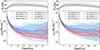 |
Fig. B.1. Evolution of median DM (left bottom panel) and gas (right bottom panel) density of the environment around dark and bright galaxies. Dark galaxies are shown as dotted-dashed lines, and bright galaxies as solid lines. Each colour represents a different simulation, blue shades for HESTIA and red for NIVARIA-LG. The shaded and striped backgrounds are the regions limited by the 16th and 84th percentiles of the distributions. The environment is defined as a spherical shell between 1 Rvir and 7 Rvir of each halo at each time. The evolution of the median Rvir of all dark and bright galaxies is shown in the top panels as a solid black line, along with the 16th and 84th percentiles as a shaded region. |
All Tables
All Figures
|
Fig. 1. M★–Mhalo relation for isolated galaxies within our simulated Local Group analogues, containing gas and stars and with DM halo masses between 109 M⊙ and 1012.5 M⊙. Galaxies from the HESTIA simulations are coloured in shades of blue, and galaxies from NIVARIA-LG in red. The M★ − Mhalo relations from Moster et al. (2013), Brook et al. (2014), and Girelli et al. (2020) are shown in dotted-dashed, dashed, and dotted lines, respectively. |
| In the text | |
|
Fig. 2. Number of galaxies from the four simulations as a function of the DM halo mass (left panel). The total sample of dark galaxies is shown in magenta and the total sample of bright galaxies is shown in green. The right panels show the same distributions separately for HESTIA simulations in blue (top) and for NIVARIA-LG simulations in red (bottom), representing dark and bright galaxies with dotted-dashed and solid lines, respectively. |
| In the text | |
|
Fig. 3. M★–Mhalo relation (top), gas-to-halo mass relation (centre), and H I-to-halo mass relation (bottom), for dark (filled markers) and bright (empty markers) galaxies at z = 0. Galaxies from the HESTIA simulations are coloured in shades of blue and galaxies from NIVARIA-LG are in red. Circles indicate dark galaxies with stars, whereas squares indicate starless dark galaxies. In the top panel, the M★–Mhalo relations from Moster et al. (2013), Brook et al. (2014), and Girelli et al. (2020) are shown in dotted-dashed, dashed, and dotted lines, respectively. We include Cloud-9 as a black diamond in the top and bottom panels. |
| In the text | |
|
Fig. 4. Evolution of the median DM halo masses of dark galaxies (dotted-dashed lines) and bright galaxies (solid lines) as a function of redshift. Red lines represent the median of all galaxies of the NIVARIA-LG simulation, whilst blue lines correspond to the median of all galaxies for the HESTIA runs. The red and blue dots indicate the redshifts at which the galaxies reach half of their final halo mass. Following the scheme from Benitez-Llambay & Frenk (2020), we show with the dotted-dashed grey line the critical mass needed for gas to collapse. In addition, the dashed cyan line shows the critical halo mass for a fixed virial temperature of Tb = 2 × 10⁴ K. The dashed orange line represents the halo mass above which atomic hydrogen cooling is efficient. |
| In the text | |
|
Fig. 5. Concentration-halo mass relation for dark (filled markers) and bright (empty markers) galaxies at z = 0, colour-coded as in Fig. 3. The dashed black line is the c200 relation drawn from Dutton & Macciò (2014), and the dotted-dashed grey line represents a lineal fit of both the dark and bright sample together, i.e. log10(cNFW) = − 0.01 log10(Mhalo/M⊙)+1.27. The shaded region shows the 3σ scatter of both relations. |
| In the text | |
|
Fig. 6. Probability density distribution of the spin parameter of the DM halo, P(λ), for dark galaxies in magenta and bright galaxies in green in all four simulations. The vertical dashed lines indicate the median values for each distribution, being λdark = 0.036 ± 0.003 for dark galaxies, and λbright = 0.026 ± 0.002 for bright galaxies. The solid grey line represents the log-normal fiducial distribution from Bullock et al. (2001), and the dashed grey line indicates its median, i.e. λ0 = 0.035 ± 0.005. |
| In the text | |
|
Fig. 7. Temperature-density diagram for gas particles in all dark (top row) and all bright (bottom row) galaxies. Each column corresponds to a different simulation, from left to right HESTIA 09_18, 17_11, 37_11, and NIVARIA-LG. The horizontal dashed line indicates the threshold temperature below which gas is able to form stars in NIVARIA-LG, whilst the vertical cyan and white lines show the corresponding density thresholds to set off SF in HESTIA (nth = 0.13 cm−3) and NIVARIA-LG (nth = 10 cm−3), respectively. The continuous red line in the T − ρ diagrams of dark galaxies corresponds to the predicted temperature-density relation expected in RELHICs, as derived in Benítez-Llambay et al. (2017). Note that the dark galaxy histogram corresponding to HESTIA 37_11 is rather sparse, as only one object of this type is found in that simulation. |
| In the text | |
|
Fig. 8. Projected positions of dark (magenta) and bright (green) galaxies in the x − y (top row) and x − z (bottom row) planes at z = 0, within a sphere of 2.5 Mpc of radius from the MW. From the left to right, we present the three HESTIA simulations (09_18, 17_11, and 37_11) and NIVARIA-LG. Circles indicate dark galaxies with stars, whereas squares indicate the starless dark galaxies. The background shows the density of DM in orange and the gas density in yellow. The region is centred on the MW, shown as a blue triangle, while M31 is represented as a blue cross mark. |
| In the text | |
|
Fig. 9. Cumulative distribution of the radial distances of dark (magenta) and bright (green) galaxies with respect to the MW analogues for all four simulations at z = 0. The horizontal grey line marks the mean of the distributions, while the two vertical lines indicate the distances within which 50% of dark and bright galaxies are found, corresponding to rMW = 1.9 Mpc and rMW = 1.3 Mpc, respectively. |
| In the text | |
|
Fig. 10. Evolution of median DM (left panel) and gas (right panel) density of the environment around the full sample of dark galaxies in magenta and bright galaxies in green, combining all four simulations. The shaded backgrounds are the regions limited by the 16th and 84th percentiles of the distributions. The environment is defined as a spherical shell between 1 Rvir and 7 Rvir of each halo, at each redshift. |
| In the text | |
|
Fig. 11. Mass of H I versus DM halo mass for dark galaxies in each simulation, with HESTIA indicated as blue shades, while NIVARIA-LG is shown in red. Squares denote starless dark galaxies. The grey shaded regions represent galaxies with H I masses that could be detectable with FAST in 1 hour of integration time and at distances of < 1 Mpc and < 2.5 Mpc from the MW analogues. The concentric circles indicate dark galaxies whose central H I column densities exceed the FAST detection limit, NH I. We include Cloud-9 as a black diamond. |
| In the text | |
|
Fig. 12. H I mass versus radial distance of dark galaxies with respect to the MW analogues in each simulated run, with HESTIA indicated as blue shaded symbols and NIVARIA-LG as red symbols. Squares correspond to starless dark galaxies. The dotted-dashed grey line represents the minimum H I mass that galaxies must have to be detectable by FAST, as a function of their distance from us. Dark galaxies likely to be detectable by FAST are those that fall within the shaded region. The concentric circles indicate dark galaxies whose central H I column densities NH I exceed the FAST detection limit. Cloud-9 is included as a black diamond at d = 4.7 Mpc. |
| In the text | |
|
Fig. 13. H I column density profiles of dark galaxies for the HESTIA simulations (left) and the NIVARIA-LG simulations (right), coloured by H I mass. The dotted-dashed grey line represents the minimum H I column density value that FAST can reach, which is NH I = 2 × 1017 cm−2. The coloured shaded area in each panel shows the softening length corresponding to each simulation. A smaller number of dark galaxies could be detected by the less sensitive ALFALFA Survey, whose sensitivity is NH I ≳ 2 × 1018 cm−2. |
| In the text | |
|
Fig. B.1. Evolution of median DM (left bottom panel) and gas (right bottom panel) density of the environment around dark and bright galaxies. Dark galaxies are shown as dotted-dashed lines, and bright galaxies as solid lines. Each colour represents a different simulation, blue shades for HESTIA and red for NIVARIA-LG. The shaded and striped backgrounds are the regions limited by the 16th and 84th percentiles of the distributions. The environment is defined as a spherical shell between 1 Rvir and 7 Rvir of each halo at each time. The evolution of the median Rvir of all dark and bright galaxies is shown in the top panels as a solid black line, along with the 16th and 84th percentiles as a shaded region. |
| In the text | |
Current usage metrics show cumulative count of Article Views (full-text article views including HTML views, PDF and ePub downloads, according to the available data) and Abstracts Views on Vision4Press platform.
Data correspond to usage on the plateform after 2015. The current usage metrics is available 48-96 hours after online publication and is updated daily on week days.
Initial download of the metrics may take a while.