


| Issue |
A&A
Volume 710, June 2026
|
|
|---|---|---|
| Article Number | A45 | |
| Number of page(s) | 15 | |
| Section | Galactic structure, stellar clusters and populations | |
| DOI | https://doi.org/10.1051/0004-6361/202558619 | |
| Published online | 28 May 2026 | |
The chemical DNA of the Magellanic Clouds
VI. Origin and evolution of neutron-capture elements in the SMC
1
INAF – Osservatorio Astrofisico di Arcetri,
Largo E. Fermi 5,
50125
Firenze,
Italy
2
Dipartimento di Fisica e Astronomia ‘Augusto Righi’, Alma Mater Studiorum,
Via Gobetti 93/2,
40129 Bologna,
Italy
3
INAF, Osservatorio di Astrofisica e Scienza dello Spazio,
Via Gobetti 93/3,
40129
Bologna,
Italy
4
Dipartimento di Fisica, Sezione di Astronomia, Università di Trieste,
Via G. B. Tiepolo 11,
34143
Trieste,
Italy
★ Corresponding author: This email address is being protected from spambots. You need JavaScript enabled to view it.
Received:
17
December
2025
Accepted:
8
April
2026
Abstract
Context. In the context of galactic archaeology, the study of the Small Magellanic Cloud (SMC) is of crucial importance, as it represents a unique opportunity to study a nearby massive dwarf system. However, theoretical studies of the chemical evolution of this galaxy are significantly lacking.
Aims. In this study, we investigate the chemical enrichment of the SMC galaxy. In addition to the α and Fe-peak elements, we devote particular attention to the evolution of neutron-capture elements with a different origin; namely, r-process (Eu), weak s-process (Zr) and main s-process (Ba, La).
Methods. We developed chemical evolution models that use as their input the star formation histories obtained from colour-magnitude diagram fitting. We closely followed the chemical feedback provided by a large variety of nucleosynthetic sources. Our model predictions were compared with recent abundance measurements for the SMC.
Results. The developed framework aptly reproduces all the observables for elements up to the Fe-peak. The abundance patterns of n-capture elements are simultaneously reproduced only by assuming an enhanced contribution from the delayed r-process at low metallicity and a top-lighter IMF relative to the reference IMF by Kroupa 2001 (MNRAS, 322, 231). In this way, both the observed very high plateau in [Eu/Fe] and the rising trends in [s-process/Fe] ratios can be reproduced by the models.
Conclusions. This study provides, for the first time, information on the evolution of several n-capture elements in a massive dwarf irregular galaxy, also providing insight on several ingredients driving galactic evolution. Moreover, this work provides a test-bed for further modelling of the SMC in the context of the numerous surveys that will target the Magellanic Clouds in the next years.
Key words: nuclear reactions, nucleosynthesis, abundances / galaxies: abundances / galaxies: evolution / Magellanic Clouds
© The Authors 2026
 Open Access article, published by EDP Sciences, under the terms of the Creative Commons Attribution License (https://creativecommons.org/licenses/by/4.0), which permits unrestricted use, distribution, and reproduction in any medium, provided the original work is properly cited.
This article is published in open access under the Subscribe to Open model. This email address is being protected from spambots. You need JavaScript enabled to view it. to support open access publication.
1 Introduction
As the most massive satellites of the Milky Way (MW), the Large and Small Magellanic Clouds (LMC and SMC) offer the unique opportunity to study massive dwarf systems at very small distances (~50 kpc and ~62.5 kpc from the Sun, Pietrzyński et al. 2019; Graczyk et al. 2020) before Galaxy cannibalisation. In particular, the SMC, has a total mass of 2 × 10⁹ M⊙ (Stanimirovic et al. 2004). This is about one order of magnitude lower than the mass of the LMC. The stellar mass of the SMC is 5–7 × 10⁸ M⊙ (Rubele et al. 2018; Massana et al. 2022), which is comparable to the mass of the main merger of the MW, namely, Gaia-Sausage-Enceladus (e.g. Helmi et al. 2018).
The last decade has seen renewed interest in the evolution of the Magellanic Clouds, and the SMC in particular, as evidenced by several dedicated photometric surveys. These include VISTA survey of the Magellanic Clouds system (VMC; Cioni et al. 2011), SMC in Time: Evolution of a Prototype interacting late-type dwarf galaxy (STEP; Ripepi et al. 2014), Survey of the MAgellanic Stellar History (SMASH; Nidever et al. 2014), and VIsible Soar photometry of star Clusters in tApii and Coxi HuguA (VISCACHA; Maia et al. 2019). On the other hand, chemical analyses of high-resolution spectra of statistically significant samples of SMC red giant branch (RGB) stars had not been presented until very recently. The APOGEE-2 survey measured abundances for ~ 1000 SMC RGB stars, in particular Fe, α-elements (Nidever et al. 2020), Al, Ni, Ce (Hasselquist et al. 2021), and Mn (Fernandes et al. 2023). In addition, Mucciarelli et al. (2023a) presented VLT/GIRAFFE-FLAMES abundances of 14 elements (from O to La) for around ~200 SMC stars, now complemented by Anoardo et al. (2026), where Eu abundances have been presented for a comparable number of objects in the SMC.
Despite recent observations provide an almost complete chemical inventory for the galaxy, models of galactic chemical evolution (GCE) focussing on the SMC are lacking. Following the pioneering works by Pagel & Tautvaisiene (1998) and Tsujimoto & Bekki (2009) on the reproduction of the age-metallicity relation and stellar metallicity distribution observed for SMC Globular Clusters (GCs) and low-resolution observations of SMC field stars, the only exception is presented in Hasselquist et al. (2021, see their Sect. 5). However, in their work, models were built exclusively to fit the observed trends either for [Si/Fe] or [Mg/Fe], without addressing any other available constraints for the galaxy in detail. In this paper, we develop more detailed chemical evolution models for the SMC. The study of environments that evolved differently from the MW is essential to resolving uncertainties, degeneracies, and questions still present when dealing with Galactic studies (see e.g. Matteucci 2021, for a review). Among them, a striking example is represented by elements beyond the Fe-peak (A≳60) that are produced primarily by neutron (n)-capture slow (s-) and rapid (r-) processes. Indeed, the understanding of their astrophysical production sites has become one of the major topics in stellar physics and GCE (see e.g. Prantzos et al. 2020; Kobayashi et al. 2020a; Molero et al. 2023 and references therein).
On the other hand, Local Group (LG) MW satellites will be privileged targets for forthcoming multi-object spectrographs, such as 4-m Multi-Object Spectrograph Telescope (4MOST; see de Jong et al. 2019) and Multi-Object Optical and Near-infrared Spectrograph (MOONS; see Cirasuolo et al. 2020), with the Magellanic Clouds standing out in particular as the main targets of several sub-surveys (e.g. Cioni et al. 2019; Gonzalez et al. 2020). Therefore, establishing a solid modelling framework for such systems is vital in prevision of future surveys to provide a useful reference and test-bed for the data revolution (> one order of magnitude increase in the data volume; see e.g. Gonzalez et al. 2020) taking place in the next years.
In light of this, in the present work we aim at developing detailed models of chemical evolution to reproduce the SMC galaxy. Following a proper testing of the theoretical framework, based on star formation histories (SFHs) obtained by means of colour-magnitude diagrams (CMDs) from photometric surveys (Rubele et al. 2018; Massana et al. 2022), we focus on the evolution of n-capture elements in the SMC. To do so, we exploit the data from Paper I (hereafter Paper I) and Paper IV (hereafter Paper IV), where SMC abundances for Zr, Ba, La, and Eu are available. This means testing elements produced via different production channels; namely, weak s-process (Zr), main s-process (Ba and La) and r-process (Eu). In turn, this allows us to perform one of the first thorough theoretical studies on n-capture elements evolution in an environment different from that of the Galaxy. Despite the existence of several programmes targeting heavy elements in the LG (e.g. Letarte et al. 2010; Hill et al. 2019; Reichert et al. 2020 and references therein), works on the theoretical interpretation of n-capture element abundances in galaxies are either lacking or only focus on fewer elements (Ba and Eu at most; see e.g. Hirai et al. 2015; Vincenzo et al. 2015; Molero et al. 2021; Palla et al. 2025).
This paper is organised as follows. In Sect. 2, we present the framework adopted to model the chemical evolution of the SMC. In Sect. 3 we provide a brief overview of the datasets adopted for comparison with the model outputs. In Sect. 4, we compare the model predictions to the observations, focussing in Sect. 5 on the study of n-capture elements. Finally, in Sect. 6, we discuss our findings and draw our main conclusions.
2 A new chemical evolution framework for the SMC
In this section, we present the chemical evolution framework adopted for the SMC. In contrast to the approach commonly taken in the literature, where parametric forms for the gas inflows and outflows are imposed and the SFH is obtained by assuming a star formation efficiency (SFE) to convert the available gas in stars, here we consider SFHs obtained through CMD fitting (Rubele et al. 2018; Massana et al. 2022) and, by assuming a SFE for each timestep, we let the gas budget evolve accordingly to the input star formation rate (SFR).
The latter approach has the advantage of capturing variations of the SFR over small timescales, as well as tracing multiple peaks in SF and gas accretion, without implementing additional fine-tuned parameters (e.g. onset times of different SF bursts and/or gas accretion episodes, e.g. De Vis et al. 2021; Palla et al. 2024). In this way, it allows us to more readily test the different derived SFHs (see 2.1) against other galactic observables; namely, the age-metallicity relation, stellar metallicity distribution function (MDF), and [X/Fe] versus [Fe/H] patterns.
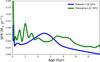 |
Fig. 1 Global SFHs for the SMC galaxy as derived by Rubele et al. (2018, blue line) and Massana et al. (2022, green line). |
2.1 Star formation histories
In this work, we adopted the SFHs inferred from SMC CMDs by Rubele et al. (2018) and Massana et al. (2022). Going into the details of the derivation of the two SFHs is beyond the scope of this work and we only provide a brief description below.
In Rubele et al. (2018, hereafter R18), the SFH across the entire main body and wing of the SMC was recovered using tile images from the VMC survey (Cioni et al. 2011) in the Y J Ks filters. The analysis was carried out in 168 sub-regions, applying a CMD reconstruction method that returns the best-fitting SFR(t) (with an age–metallicity relation, distance and mean reddening; see Rubele et al. 2015). In Massana et al. (2022, hereafter M22), the SFH of the SMC was obtained by using deep u g riz photometry of the second data release of the SMASH survey instead (Nidever et al. 2021). Their analysis was performed on 74 sub-regions with a similar number of stars using Voronoi binning (Cappellari & Copin 2003) and applying a CMD reconstruction method for the SFH of the galaxy.
Since the focus of our work is on the SMC integrated properties, for both studies, we used integrated SFHs by summing up the contribution of each sub-region at each timestep. Moreover, it is worth noting that, as in R18, the SFH is given in the form of a step function, we needed to smooth it1 to obtain a more realistic behaviour of the SFR with time. This procedure is not necessary for M22, as they already provided a smoothed final solution for their SFH (see e.g. Ruiz-Lara et al. 2018, for details).
The resulting SFHs as functions of age or lookback time are shown in Fig. 1. They display a quite different evolution, with R18 exhibiting a smoother behaviour relative to M22, which displays much more prominent SF peaks, especially at recent times (age ≲2–3 Gyr). This marked increase in SF around 3 Gyr ago in M22 was also observed in previous analyses (e.g. Harris & Zaritsky 2004) and is associated with interactions or close encounters with the LMC. These would also trigger the present-time SF burst observed by both R18 and M22. On the other hand, the higher SFR at older ages in M22 can be attributed by the authors to the magnitude limit of the VMC survey, as the 10 Gyr old main sequence turnoff lies very close to the 50% VMC completeness limit. The differences in the SFHs inferred by R18 and M22 are also reflected in the stellar masses integrated over the galaxy lifetime (5.2 • 108 M⊙ for R18, 6.7 • 108 M⊙ for M22); whereas the timescales for stellar mass accumulation are similar (50% of the stellar mass formed in the first ≃8.5 Gyr).
2.2 Chemical evolution calculations
To compute the chemical evolution of the galaxy under scrutiny, we relied on the basic equation that describes the evolution of a given element i (see e.g. Matteucci 2021), expressed as
 (1)
(1)
where the first term on the right-hand side of Eq. (1) corresponds to the rate at which an element, i, is removed from the ISM due to star formation, with the rate at a specific time, ψ(t), taken from the SFHs illustrated in Sect. 2.1.
The term Ri (see e.g. Palla et al. 2020 for the complete expression) takes into account the nucleosynthesis from different stellar sources (see Sect. 2.3 for details), weighted according to the initial mass function (IMF). The products originating from binary systems, such as Type Ia SNe and merging neutron stars, are included in Ri, while properly accounting for the respective delay-time-distributions (see Matteucci et al. 2009; Palla et al. 2025 for more details). As a reference, we adopted the IMF of Kroupa (2001) to remain consistent with the assumptions made to derive the SMC SFHs; however, we also allowed for IMF variations (e.g. Kroupa et al. 1993) to probe the impact of the latter on the galactic chemical evolution.
The last term of Eq. (1) refers to the gas flows, namely inflows and outflows. These are computed to obtain the required gas mass for a given SFR ψ(t) and SFE v(t), with the latter a free parameter of the model variable over time, in this way,
 (2)
(2)
In practice, if Mgas(t) > Mgas(t – Δt) + Ri(t – Δt), which is the gas mass at timestep t is higher than the sum of the gas mass and the returned mass from dying stars at timestep t – Δt, we impose the following condition: a gas amount equal to Mgas(t) – (Mgas(t – Δt) + Ri(t – Δt)) is accreted by the galaxy. This gas is assumed to have a primordial chemical composition. Conversely, if Mgas(t) < Mgas(t – Δt) + Ri(t – Δt), the gas excess (Mgas(t – Δt) + Ri(t – Δt)) – Mgas(t) is ejected from the system. This ejected gas has a chemical composition equal to that of the ISM at the timestep t.
2.3 Nucleosynthesis prescriptions
Among the basic ingredients of chemical evolution models are the stellar yields, namely, the amounts of different chemical elements that stars produce and eject into the ISM at their deaths. We adopted grids of stellar yields for different types of stars that have been amply tested on MW data:
For low- and intermediate-mass stars (LIMS) we adopted the set of yields for non-rotating stars available on the web pages of the FRUITY2 database (Cristallo et al. 2009, 2011, 2015).
For massive stars, we adopted the yields by Nomoto et al. (2013) that include elements up to the Fe-peak, assuming a hypernova (HN) fraction that varies with metallicity. In particular, we assume that the fraction of stars above 25 M⊙ that die as HNe is 95% up to [Fe/H] = −2.5 dex and then decreases to 0% for [Fe/H]> −1 dex. This is in line with widespread assumptions of a variable HN fraction with metallicity (e.g. Kobayashi & Nakasato 2011; Mucciarelli et al. 2021). As Nomoto et al. (2013) yields do not include those of n-capture elements, to account for the latter, we adopted the yields by Limongi & Chieffi (2018)3 In particular, we fixed set R150 (i.e. stars with uniform rotational velocity at vrot =150 km s−1) as our reference. However, in the paper we test also different sets and velocity distributions.
For Type Ia SNe, we assumed an equal mixture of near-MCh and sub-MCh progenitors. In fact, there are claims in the literature that both progenitors contribute to the chemical evolution of the Galaxy (see e.g. Kobayashi et al. 2020b; Palla 2021). The yields adopted for the two classes of progenitors were drawn from Leung & Nomoto (2018, for near-MCh) and Leung & Nomoto (2020, for sub-MCh).
To include the products of the r-process, we consider both magneto-rotational driven SNe (MRD-SNe) and merging of compact objects (MNS). For MRD-SNe we adopt the yields from model L0.75 of Nishimura et al. (2017), while for MNS we use the empirical yield measured by Watson et al. (2019) for kilonova AT2017gfo (see also Molero et al. 2023). In contrast to the yields described in previous points, the latter prescriptions do not include the dependences on the progenitor mass/metallicity. However, this is a common issue often faced when modelling the chemical evolution of the r-process elements (see Molero et al. 2025; Palla et al. 2025, and references therein).
3 Observational data
The spectroscopic data used in this work were taken from Paper I and Paper IV for field stars and from Mucciarelli et al. (2023b, hereafter Paper II) for three GCs.
Concerning the SMC field, Paper I analysed VLT/GIRAFFE-FLAMES spectra of 206 RGB stars, deriving chemical abundances for α-elements (Mg and Si), iron-peak elements (Fe and Ni), and s-process elements (Zr, Ba and La). No r-process element abundances could be derived, as the FLAMES set-ups adopted in their study did not include any transition of r-process elements. On the other hand, Paper IV measured Eu abundances from VLT/GIRAFFE-FLAMES spectra of 209 RGB stars in the SMC (158 in common with the sample of Paper I), utilising a different instrument set-up. We use the abundances of Paper IV to investigate the r-process enrichment in the SMC. Both samples cover a broad metallicity range of −2.3 ≲[Fe/H]/dex≲ −0.5, with most targets having [Fe/H]> −1.4 dex. Additionally, we included the abundances of three massive GCs in the SMC; namely, NGC 121 (the oldest SMC globular cluster, with an age of 10.5±0.5 Gyr, Glatt et al. 2008a), NGC 339 (with an age of 6±0.5 Gyr, Glatt et al. 2008b), and NGC 419 (with an age of 1.4±0.2 Gyr, Glatt et al. 2008b). All of them were analysed using VLT/UVES-FLAMES (II). This is the only sample of chemical abundances for SMC clusters derived from high-resolution spectroscopy and it provides a time-resolved reconstruction of the chemical enrichment history of the SMC.
4 Reproducing the main SMC chemical properties
In the following, we present the predictions of the chemical evolution models described in Sect. 2 and their comparison with the datasets illustrated in Sect. 3.
The models adopting the two different SFHs have different star formation efficiencies, v, which have been calibrated to reproduce several observables in the galactic system; namely, the stellar metallicity distribution function (MDF), age-metallicity relation, and the [X/Fe] versus [Fe/H] patterns of chemical elements X of well-known and distinct nucleosynthetic origin (Mg, Si, Ni).
4.1 Metallicities
The age-metallicity relation predicted by the model adopting the R18 SFH was compared with the relevant data in Fig. 2 (top panel). For this model, we adopted a free parameter value of v =0.015 Gyr−1 up to an evolutionary time of t = 13 Gyr, increasing it to v =0.05 Gyr−1 in the last Gyr of evolution. The increase in the SFE can be explained in light of the large (×3–4) and rapid increase in the SFR in the last Gyr of evolution found by R18. In turn, the latter can be interpreted as a starburst stimulated by the recent interaction with the LMC. Indeed, without increasing the SFE, higher SFRs would result in larger gas accretion, which, in turn, would lead to strong gas dilution and, thus, lower metallicities than those observed in the late galactic evolutionary phases.
In Fig. 2 (top panel), the blue solid line represents the age−metallicity relation predicted by our homogeneous GCE model. The light blue points are the predictions of a synthetic model that adds a random error, equal to the typical abundance uncertainties of the data samples described in Sect. 3 (≃0.1 dex), to the abundances of the synthetic stars formed at each time, t (see also Palla et al. 2022). For each chemical element, we define a 'new abundance' of
![Mathematical equation: ${\left[ {{\rm{X/H}}} \right]_{{\rm{new}}}}\left( {\rm{t}} \right) = \left[ {{\rm{X/H}}} \right]\left( {\rm{t}} \right) + N\left( {\left[ {{\rm{X/H}}} \right],\sigma \left[ {{\rm{X/H}}} \right]} \right),$](/articles/aa/full_html/2026/06/aa58619-25/aa58619-25-eq3.png) (3)
(3)
where 𝒩 is a random function with normal distribution. In this way, we were able to ensure a fair comparison between the model predictions and the observations, avoiding any artificial discrepancy caused by data uncertainties. Our model predictions are well aligned with both the SMC GC data of Paper II and the theoretical relation of Pagel & Tautvaisiene (1998). The only significant difference between the relation by Pagel & Tautvaisiene (1998) and ours is found at ages comprised between 2 and 4 Gyr, where our model predicts metallicities up to ~0.4 dex higher. Unfortunately, no high-resolution data are available for GCs in this age range. Previous low-resolution works (Parisi et al. 2009, 2015, 2022; Dias et al. 2021) offer a very broad metallicity spread. This type of spread in low-resolution data has also been observed for younger GCs (ages ~1 Gyr), with some of the clusters reaching [Fe/H] values lower than both the GC NGC 419 observed at high-resolution and model predictions by almost 0.5 dex. A possible explanation of the metallicity spread could reside in clumpy SF within the SMC late evolution, as can be inferred from the particular galaxy morphology (e.g. Zaritsky et al. 2000; Martínez-Delgado et al. 2019).
In Fig. 2 (bottom panel), we compare the predicted MDF with the observed ones from Paper I and APOGEE DR17 (Hasselquist et al. 2021). The model distribution peaks at [Fe/H] slightly below −1 dex, akin to the observed distributions, also showing a very similar median: < [Fe/H] >model= −1.06 dex, < [Fe/H] >APOGEE = −1.07 dex, < [Fe/H] >M23= −1.04 dex (see the dashed lines in the figure). The only visible discrepancy between observations and model outcome resides in the metal-rich tail of the MDF, where predictions show a slightly higher fraction of stars than both Paper I and APOGEE distributions.
In Fig. 3 (top panel), the age-metallicity relation predicted by the model adopting the M22 SFH is compared with the relevant data. In this case, we adopted a SFE value of v =0.01 Gyr−1 up to t = 11 Gyr, increasing it to v =0.05 Gyr−1 in coincidence with the multiple bursts of SF observed by Massana et al. (2022) in the last 3 Gyr. The adoption of a higher SFE allowed us to reproduce the metallicity of the young SMC GC NGC 419 that otherwise would be underestimated, as a large increase in the average SFR would imply significant gas dilution if not accompanied by an increase in the star formation efficiency. In general, we note that the model adopting M22 SFH produces metal-richer stars at intermediate ages (4–8 Gyr) relative to the model adopting R18 SFH. However, the model with M22 SFH also results in lower metallicities at younger ages (≲4 Gyr), which further highlights the effect of SF peaks in metallicity dilution as due to the injection of fresh gas into the galaxy ISM. Despite the differences relative to the R18 SFH model, the general trend shown by the observations is still well matched, with the synthetic model adopting M22 reproducing the abundances of SMC GCs observed both at high- and low-resolution. The predicted MDF (green histogram in Fig. 3, bottom panel) reflects the differences highlighted in the age-metallicity relation: the distribution shows a peak skewed towards metal-rich stars, between −0.9 and −1 dex in [Fe/H]. This is still in good agreement with APOGEE and Paper I observations. At the same time, predictions do not reveal an excess of stars in the metal-rich tail ([Fe/H] ≳ −0.8 dex) as for R18; rather, they suggest a slight overabundance in metal-poor stars (−1.5 ≲[Fe/H]/dex≲ −1.3). Nevertheless, the model distribution aligns well with the observations, with a median value (< [Fe/H] >model= −1.04 dex) that is close to what is given by the data (< [Fe/H] >APOGEE = −1.07 dex, < [Fe/H] >M23= −1.04 dex).
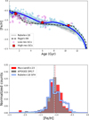 |
Fig. 2 Age-metallicity relation (top panel) and MDF (bottom panel) as predicted by the reference chemical evolution model adopting Rubele et al. (2018) SFH (blue line, circles and histogram, respectively). The predicted age-metallicity relation is compared with the CMD-extracted relation by Rubele et al. (2018, grey line with confidence intervals), the theoretical curve by Pagel & Tautvaisiene (1998, bursting model, black dashed line), SMC GCs from low-resolution (Parisi et al. 2009, 2015, 2022; Dias et al. 2021, magenta empty circles) and high-resolution studies (Mucciarelli et al. 2023b, red filled squares). Observed MDFs are from Mucciarelli et al. (2023a, red histogram) and Hasselquist et al. (2021, APOGEE DR17, grey histogram). |
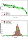 |
Fig. 3 Age-metallicity relation (top panel) and MDF (bottom panel) as predicted by the reference chemical evolution model adopting Massana et al. (2022) SFH (green curve, circles and histogram, respectively). Data are as in Fig. 2. |
4.2 α and Fe-peak elements abundance patterns
Another necessary step to test the models is to look at [X/Fe] versus [Fe/H] diagrams for elements with a well-known nucle-osynthetic origin for which we already have solid predictions in the context of the MW and the solar vicinity. Building on the sample of available elements in Paper I, we looked at Mg, Si, and Ni. These three elements are synthesised by means of different processes and stellar sources and timescales: Mg is mainly produced by hydrostatic burning in massive stars (Woosley & Weaver 1995), Si is made during explosive burning in massive stars with non-negligible contribution from Type Ia (Romano et al. 2010; Kobayashi et al. 2020a and references therein), and Ni is primarily produced by Type Ia SNe (Kobayashi et al. 2020b; Palla 2021 and references therein). Moreover, the [X/Fe] versus [Fe/H] patterns for Mg, Si and Ni observed by Paper I are very similar to the ones in APOGEE (Hasselquist et al. 2021, see Fig. A.1), ruling out spurious patterns due to particular observational biases.
The comparison between the predictions of the models adopting R18 SFH and M22 SFH and the observed abundance trends for Mg, Si, and Ni are shown in Fig. 4 (left, central, and right panels, respectively). Both models show a good agreement with the bulk of the observed abundances: the predictions of our synthetic models (see Sect. 4.1) aptly cover the regions representing most of the data (red contours in Fig. 4). Indeed, it is worth noting that the predicted [X/Fe] versus [Fe/H] patterns for the models adopting R18 and M22 SFHs are basically indistinguishable when considering abundance uncertainties, with (rather small) differences arising only when looking at the homogeneous model tracks (see discussion in Romano et al. 2015). As a further check for the models, the predicted abundances were also compared with SMC GCs high-resolution observations by Paper II: [Si/Fe] and [Ni/Fe] abundances (we did not consider Mg due to the Mg-Al anti-correlation in GCs, Gratton et al. 2012) are well aligned with the model outcome, confirming what already been seen for SMC field stars.
Therefore, despite small residual differences between model predictions and observations, the average age-[Fe/H], MDF, and [X/Fe] versus [Fe/H] patterns are well reproduced, indicating that we have built a solid framework to probe the evolution of n-capture elements in the SMC (see the next section). Indeed, the understanding of the nucleosynthetic origin of such elements is still limited (e.g. Molero et al. 2023, 2025; Palla et al. 2025), making uncertainties about elemental nucleosynthesis much more relevant than the small discrepancies encountered in this section.
5 n-capture elements in the SMC
Here, we focus on the evolution of n-capture elements Zr, Ba, La, and Eu, obtained in the observations described in Sect. 3. It is important to note that the four elements belong to different families, to which different production mechanisms correspond: Zr (Z=40) belongs to the first s-process peak, for which the predominant mechanism is the weak s-process in rotating massive stars (e.g. Pignatari et al. 2010; Limongi & Chieffi 2018); Ba (Z=56) and La (Z=57) are second peak s-process elements, where the main s-process mechanism in low-mass AGB stars is predominant (e.g. Cristallo et al. 2015); and Eu (Z=63) is a pure r-process element (e.g. Burris et al. 2000; Sneden et al. 2008).
Therefore, the comparison performed in this section represents the first attempt to model a representative number of n-capture elements with different origin simultaneously in the SMC, and in general in LG galaxies beyond the metallicity regime dominated by stochastic enrichment; namely, at [Fe/H]≲ −2 (e.g. Schönrich & Weinberg 2019). Indeed, previous theoretical works on LG dwarfs have focussed on Ba or Eu alone (e.g. Hirai et al. 2015; Vincenzo et al. 2015) or Ba and Eu at most (Molero et al. 2021, for Fornax, Sculptors dSphs and Reticulum II UFD). Furthermore, earlier works were based on older prescriptions concerning s- and r-process nucleosynthesis, which have seen several revisions during recent years with relevant effects on well-known Galactic patterns (see e.g. Prantzos et al. 2020; Molero et al. 2023).
In Fig. 5, we show the model predictions for n-capture elements for both the models using R18 and M22 SFHs, adopting the n-capture element set-up as described in Molero et al. (2023). This set-up (r-process sources, yields, and delay times, as well as s-process sources and yields; see also Sect. 2) allowed us to reproduce the Galactic observables, from abundance patterns in r- and s-process elements to the measured MW event rates (see Molero et al. 2023; Palla et al. 2025).
Nonetheless, Fig. 5 clearly shows that the adopted enrichment set-up for n-capture elements fails to reproduce the observed patterns in the SMC. Indeed, all the elements under scrutiny are severely underestimated, even accounting for abundance uncertainties with our synthetic framework. In addition, models adopting different SFHs show minimal variations in terms of their abundance patterns for all these elements. For this reason, for the rest of the paper, we focus the model predictions obtained from R18 SFH (but see Fig. C.1), to facilitate the comparison between data and models. It is worth noting that a deficiency in Eu production in the LG by GCE models was noted in Palla et al. (2025) for the Sagittarius, Fornax, and Sculptor dwarf galaxies. However, here we note that a similar deficiency is also present for other n-capture elements for which the s-process should be the main production mechanism (e.g. Prantzos et al. 2020). Therefore, in the following we try to reconstruct the origin of this discrepancy by analysing several pathways to recover this missing production process.
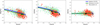 |
Fig. 4 X/Fe] vs [Fe/H] for light elements in the SMC. Abundance patterns are shown for Mg (left panel), Si (central panel) and Ni (right panel) for reference models adopting Rubele et al. (2018) SFH (blue lines and cyan regions) and Massana et al. (2022) SFH (green lines light-green regions). Solid lines are genuine chemical evolution tracks for models with a given SFH, whereas shaded regions are associated model predictions account for observational uncertainties (i.e. synthetic model). Data come from Mucciarelli et al. (2023a, SMC field stars, orange dots) and Mucciarelli et al. (2023b, SMC GCs, black squares). The orange contour lines represent the density lines of the observed stellar distributions in SMC field stars. |
 |
Fig. 5 [X/Fe] vs [Fe/H] for n-capture elements in the SMC. Abundance patterns are shown for Eu (left-most panel), Zr (second left-most) and Ba (second right-most) and La (right-most). Solid lines show the genuine chemical evolution tracks for the reference models adopting Rubele et al. (2018) SFH (blue) and Massana et al. (2022) SFH (green). The shaded cyan and light-green regions are associated model predictions account for observational uncertainties (i.e. synthetic models). Data come from Anoardo et al. (2026, Eu) and Mucciarelli et al. (2023a, Zr, Ba, La) for SMC field stars (orange dots) and Mucciarelli et al. (2023b) for SMC GCs (black dots). The orange contour lines represent density lines of the observed stellar distributions in SMC field stars. |
5.1 Increased r-process production at low-metallicity
As a first step, we focussed on Eu, which is a pure r-process element, meaning that is (almost) only produced by means of the r-process (Burris et al. 2000; Sneden et al. 2008). In this way, we isolated one production channel that still has a non-negligible contribution in the nucleosynthesis of Zr, Ba and La (≃19%, 14%, and 24% at solar, Sneden et al. 2008).
As mentioned earlier in this paper, Palla et al. (2025) noticed a lack in [Eu/Fe] (≳0.5 dex) for GCE models of several LG dwarfs, suggesting that 3/4 of the needed Eu production in dwarf galaxies is missing, despite the adopted prescriptions reproduce the observed MW patterns. To reconcile the discrepancy between the Galactic and extragalactic observations, they suggested a marked increase in Eu production by MNS events at low metallicity. In particular, they adopted a variable fraction of stars that originate MNS events (αMNS) via
 (4)
(4)
where αMNS,0 = 2 • 10−3 and Zthresh = 2 • 10−3 ≃ 0.1 Z⊙.
Therefore, we applied the same formulation as in Eq. (4) to our chemical evolution model for the SMC. This is shown in Fig. 6. As we note in the left panel, the boost in Eu production by MNS produces a significant rise in the [Eu/Fe] abundance, with a plateau extending up to metallicities slightly above [Fe/H] = −1 dex. The extended plateau is the effect of the large Eu production rate by MNS originating up to the given metallicity threshold. After the metallicity threshold for enhanced Eu production is passed and the enhanced production progressively fades, the [Eu/Fe] ratio declines with metallicity due to an unbalanced production of Fe (mainly by Type Ia SNe) relative to Eu. In any case, the new predicted trend for Eu remains in part below the bulk of SMC stars, especially for metallicities below [Fe/H] ~ −1 dex.
A significant reduction in the offset observed in Fig. 5 can also be seen for the three s-process elements in the three rightmost panels of Fig. 6. Despite being dubbed as s-process elements, Zr, Ba, and La receive a fundamental contribution from r-process at low-metallicities, where s-process production is disfavoured by the low-metallicity environment (due its secondary nature4) and/or the longer lifetimes of the stellar production sources (low-mass stars). However, we find, especially for Ba and La (where the s-process production is dominated by low-mass stars via the main s-process), a clear [X/Fe] deficit in the predictions: the model does not show the expected increase in the [s-process/Fe] ratio driven by low-mass stars at high-metallicity (Molero et al. 2023, and references therein). Instead, it exhibits a flat trend that prevents most of the SMC field stars and GCs data from being covered. It is worth noting that for all the n-capture abundance patterns in Fig. 6, analogue results are found for the M22 SFH, as shown by Fig. C.1. This further confirms the small differences in terms of [X/Fe] versus [Fe/H] patterns by the two SFHs, even in the presence of nucleosynthesis prescriptions dependent on galactic SF and chemical enrichment.
In summary, the increase in MNS r-process production at low metallicities, as proposed in Palla et al. (2025) clearly helps to reconcile the predictions with observations of n-capture elements. However, we still fall short in explaining several of the features described by the observed abundance patterns in the galaxy.
 |
Fig. 6 [X/Fe] vs [Fe/H] for n-capture elements for the model adopting Rubele et al. (2018) SFH with increased MNS r-process production at low-metallicity (see Eq. (4)). Blue solid lines and cyan shaded regions represent genuine chemical tracks and model predictions accounting for observational uncertainties ('synthetic model'), respectively. Data are as in Fig. 5. |
5.2 Impact of the IMF
Up to this point in the study, we adopted the IMF by Kroupa (2001) to be consistent with the adopted SFHs, derived by assuming the same IMF. However, it is worth exploring whether variations in the IMF can significantly influence the evolution of n-capture elements in the SMC. Indeed, the IMF regulates the relative fractions of low- and high-mass stars within stellar populations, which has a critical impact on the metal production and abundance ratios in galaxies. In addition, several indications (e.g. Lee et al. 2009; Watts et al. 2018) point towards steeper (or toplight) IMFs in the high-mass domain in dwarf galaxies; namely, by reducing the relative fraction of massive stars. These can be framed in the context of the integrated galactic IMF (IGIMF) theory, where galaxies with lower rates of star formation are prone to underproduce massive stars (e.g. Jerábková et al. 2018; Yan et al. 2020).
Therefore, in this section, we focus on testing the effect of different IMFs from the canonical one (Kroupa 2001, high-mass end slope x = −1.3), by adopting the Kroupa et al. (1993) IMF formulation (x = −1.7) or a modification of the latter with an even steeper slope (hereafter dubbed 'top-light', x = −2). It is worth remarking that our test is not driven by the intention to dig deeper into the intricate debate about the IMF (see Jerabkova et al. 2025) and we know that different assumptions in the IMF can produce differences in the extracted SFHs. However, Figs. 4 and 5 demonstrate relatively small differences in the abundance patterns obtained by means of different SFHs for the galaxy, with other ingredients being more relevant in shaping [X/Fe] versus [Fe/H] diagrams. In any case, since the change in the IMF has consequences not only for the production of n-capture elements, but also the global metal evolution, all the models adopting an IMF different from the canonical one were re-calibrated in the SFE v to reproduce the main SMC observables, as in Sect. 4 (see Appendix B). In this way, we were able to avoid spurious results arising from chemical evolution histories inconsistent with observations.
The [X/Fe] versus [Fe/H] patterns for Eu, Zr, Ba, and La for models with enhanced MNS r-process production, adopting the Kroupa et al. (1993) IMF and the top-light IMF are shown in Fig. 7, together with the one assuming the canonical Kroupa (2001) IMF. For the model with the top-light IMF, we also show the prediction from the synthetic framework (see Sect. 4).
The figure shows that the proposed change in the IMF has a beneficial effect in the reproduction of the abundance patterns. For [Eu/Fe] (Fig. 7 leftmost panel), the predicted behaviour for the model with top-light IMF remains similar to the one shown in Fig. 6. However, the plateau at lower metallicities is shifted to higher values (~0.5 dex, difference ~0.25 dex from the model with the canonical IMF). This happens because the models adopting top-lighter IMFs need for larger SFE to reproduce the SMC observables, increasing the contribution to r-process enrichment by MRD-SNe. In turn, when abundance uncertainties are considered, this allowed us to reproduce most of the observed field stars and GCs in the SMC.
For [Zr/Fe], displayed in Fig. 7 (second left-most panel), the predictions from the models show an extended plateau similar to Eu, but at roughly solar [Zr/Fe] values for models adopting the steeper IMFs. Then, the models reveal a small rise between [Fe/H] ~ −1.25/−1 dex, due to increased s-process production mostly by (rotating) massive stars caused by the peak in SF at intermediate ages (see Fig. 1), followed by a gentle decline at the highest metallicities as a consequence of Type Ia SN enrichment. Also in this case, the adoption of a steeper IMF greatly helps to reproduce the general trend captured by the data. Again, this happens for the rise in SFE for models with steeper IMF slopes. In the present case, it causes not only the r-process with MRD-SNe to increase, but also the weak s-process channel through massive stars.
However, it is in the case of Ba (Fig. 7 in the second rightmost panel) that the adoption of an IMF favouring (disfavouring) the presence of low-mass (massive) stars is shown to be the most beneficial. In fact, the top-light IMF not only allows for an upward shift in the low-metallicity plateau, but also for a rise in [Ba/Fe] from metallicties [Fe/H] ≳ −1.25 dex. The latter is the direct consequence of the larger weight of low-mass stars in chemical enrichment, as Ba (and La as well) is preferentially produced through the main s-process in low-mass (~1–3 M⊙) stars. This increase in [Ba/Fe] abundance with metallicity, despite being not very large (~ 0.25 dex), is crucial to recovering a good agreement with the bulk of field star and GC data, which otherwise would remain underestimated by models. The rise with metallicity offers an important aid in the data-model agreement also for [La/Fe] (Fig. 7 right-most panel). However, despite the substantial improvement in reproducing the observed La, part of the data remains above the predictions, even when accounting for observational errors.
To probe the evolution of heavy elements more in detail and, in particular, the relative contribution between the r-process and s-process channels, in Fig. 8 we show the predicted mass fraction evolution of s-process component (top panels) and [X/Eu] abundance ratios as a function of metallicity compared with the samples described in Sect. 3 (bottom panels). Figure 8 (bottom panels) shows a good agreement between observation and predictions. The model adopting a top-light IMF nicely reproduces the trends observed in [Zr,Ba,La/Eu], with data superimposed to predictions in our synthetic GCE framework.
In particular, Zr shows a flat/slowly increasing trend relative to Eu, denoting a relevant r-process contribution throughout galactic evolution. Indeed, the s-process fraction evolution for Zr (top left panel in Fig. 8) denotes a sub-dominant production through the s-process channel, with a mass fraction of the order of 0.4 at the present day. In contrast, we observe larger s-process contribution for Ba and La (two rightmost panels on top) with present-day values of ~0.7–0.8 for both elements, obtained by a progressive increase throughout Gyr. The increase in s-fraction is also visible in the [Ba,La/Eu] versus [Fe/H] patterns in Fig. 8 bottom panels, with a sharp rise in [X/Eu] starting from [Fe/H] ~ −1.25 dex up to the highest predicted metallicities. This is a consequence of delayed enrichment by low-mass stars, whose contribution is the dominant channel for main s-process elements (as Ba and La).
This is also demonstrated by the lower s-process fractions by models adopting an IMF favouring massive star production (see the dashed and dash-dotted lines in the upper panels). For Ba and La, the s-channel contribution at present-day is reduced by more than 30% by adopting a Kroupa (2001) IMF, almost halving the role of the s-process in the synthesis of elements. A reduction in the s-process fraction is also seen for Zr, but here of a 10% only. Moreover, the decrease for Zr is mostly driven by the lower contribution from massive stars, due to the lower SFE in the models adopting top-heavier IMFs (see earlier in this section).
 |
Fig. 7 [X/Fe] vs [Fe/H] for n-capture elements for the model with Rubele et al. (2018) SFH and increased MNS r-process production at low-metallicity (see Eq. (4)), adopting different IMFs. Blue lines represent models adopting the reference Kroupa (2001) IMF (thin dash-dotted), Kroupa et al. (1993) IMF (thin dashed) and a Kroupa et al. (1993) IMF with steeper high-mass end slope (top-light IMF, thick solid). Cyan shaded regions show the predictions for the model with top-light IMF, accounting for observational uncertainties ('synthetic model'). Data are as in Fig. 5. |
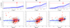 |
Fig. 8 Mass fraction produced by the s-process channel of production (top panels) and [X/Eu] vs [Fe/H] (bottom panels) for Zr (left panels), Ba (central panels) and La (right panels) for models with different IMFs. In the top panels, we show the results for models adopting the reference Kroupa (2001) IMF (thin dash-dotted lines), Kroupa et al. (1993) IMF (thin dashed), and a modified a top-light IMF (thick solid). In the bottom panels, blue solid lines an cyan shaded regions are genuine chemical tracks and predictions accounting for observational uncertainties ('synthetic model') for a model with a top-light IMF. Data include the Solar s-process mass fraction (Sneden et al. 2008, top panels) and those shown in Fig. 5 (bottom panels). |
5.3 Different IRV distribution for massive stars
Other possible explanations for the observed abundance patterns in n-capture elements might also be considered. In particular, considering the s-process, the initial rotation velocity (IRV) distribution in massive star populations is an active object of study (e.g. Rizzuti et al. 2019; Prantzos et al. 2020; Molero et al. 2025). For our reference yield set for massive star s-process production (Limongi & Chieffi 2018 set R150), we adopted a fixed initial rotational velocity of 150 km s−1. Even though such a prescription is observationally motivated, as it allows for Galactic observations to be reproduced for a large number of n-capture elements (see Molero et al. 2023), the adoption of sets with different rotational velocities (for Limongi & Chieffi 2018, vrot = 0, 300 km s−1 ) or a distribution of velocities is worth consideration.
Therefore, alongside the reference yield set R150, we chose to consider additional sets. We tested individual sets (Limongi & Chieffi 2018 set R300, vrot = 300 km s−1) and distributions of rotational velocities that vary with metallicity. For the latter, we adopted the distributions as in Molero et al. (2024, hereafter DIS2) and Romano et al. (2019, hereafter DIS3), both assuming that the probability that a star rotates at a certain speed is a function of the metallicity, Z, with higher velocities being more likely at lower Z (see Table 1 for details). This is supported by the expectation that massive stars rotate faster at lower metallicities, where they are more compact (see Klencki et al. 2020). This view is supported both theoretically and observationally (e.g. Frischknecht et al. 2016; Martayan et al. 2007b,a; Hunter et al. 2008; see Molero et al. 2024 for a discussion). It is worth mentioning that other IRVs to those shown in Table 1 can be considered. However, exploring in detail the IRV of massive stars in the SMC goes beyond the scope of this paper, with other literature distributions either showing more extreme [X/Fe] patterns (at odds with observations) or very similar results to the set-ups displayed in Table 1.
The predicted [Zr,Ba,La/Fe] versus [Fe/H] chemical tracks for models adopting a Kroupa (2001) IMF and the massive stars IRV distributions given in Table 1 are shown in Fig. 9. In particular, models with R300, DIS2 and DIS3 distributions show enhanced [X/Fe] relative to the reference yields adopted in this paper. Going more into detail, the model with all stars rotating at vrot = 300 km s−1 (R300, dashed lines) overestimates the predicted trends relative to the observations, indicating an excess of s-process production by high-speed rotators when assumed as the sole contributors to the weak s-process channel. Indeed, when assuming that only a fraction (decreasing with metallicity) of massive stars are high-velocity stellar rotators (DIS2, dash-dotted lines) the [X/Fe] enrichment level generally decreases, with predictions more in agreement with observations, especially for Zr and La. A fairly good agreement between models and observations can also be seen for the model adopting the DIS3 IRV distribution (dotted lines), where a decreasing trend in the [s-process/Fe] ratios can be observed, starting from [Fe/H]≃ −2 dex. This is due to the progressive cease of contribution from vrot = 300 km s−1 rotators for metallicities beyond [Fe/H] = −2 dex. In turn, this allowed us to reproduce well the observed decreasing [Zr/Fe] trend, whereas it is at odds with the observed increase in Ba with metallicity.
As highlighted in Sect. 5.2, a more detailed look can be achieved by looking at [X/Eu], a proxy to indicate the fractional contribution from the s- and r-processes throughout galactic evolution. For this reason, in Fig. 10, we show the [X/Eu] abundance ratios as function of the metallicity (bottom panels) and the mass fraction evolution of s-process (top panels) for Zr, Ba, and La. All models display very high s-process mass fractions with values ≳0.6 already at 2 Gyr of evolution, especially for Ba and La. This is also reflected in the predicted [X/Eu] patterns (shown in Fig. 10 for the DIS2 distribution), which lie above the abundances observed in the SMC stars. Indeed, even by postprocessing the output of the model with abundance uncertainties, the predictions are only able to reproduce the upper envelope of the data. Similar (or even worse) results for comparisons in abundance patterns were observed for the other distributions tested, reaching an overestimation in [X/Eu] of the order of 0.5–0.75 dex relative to the observations in the case of the R300 model, which shows the largest s-process fraction (≳0.8 at 2 Gyr of evolution).
In summary, the contribution of high-speed rotators (vrot = 300 km s−1 ) should be marginal to reproduce the observed trends in the SMC, at least with the yield sets by Limongi & Chieffi (2018). This is also the case when using the other IMFs, as described in the previous section (Kroupa et al. 1993, top-light). In fact, despite not favouring the presence of massive stars in a stellar population as for the reference IMF, the higher SFE adopted for steeper IMF slopes (see 5.2) has the effect of keeping (where not, in fact, increasing) the contribution from rotating massive stars to the s-process enrichment constant (see Fig. C.2).
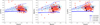 |
Fig. 9 [X/Fe] vs [Fe/H] for Zr, Ba, and La for the model with Rubele et al. (2018) SFH and increased MNS r-process production at low-metallicity (see Eq. (4)), adopting different IRV distributions (see Table 1). Blue lines represent models adopting the reference IRV distribution (R150, thick solid lines), R300 distribution (thin dashed), DIS2 distribution (thin dash-dotted), and DIS3 distribution (thin dotted). Cyan shaded regions are predictions for the model with the DIS2 distribution accounting for observational uncertainties (i.e. synthetic model). Data are as in Fig. 5. |
IRV distributions for massive stars (Limongi & Chieffi 2018 models, set R) tested in this study in addition to the reference set (R150; see Sect. 2.3).
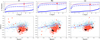 |
Fig. 10 Mass fraction produced by the s-process channel of production (top panels) and [X/Eu] vs [Fe/H] (bottom panels) for Zr (left panels), Ba (central panels) and La (right panels) for models with different IRV distributions. In the top panels, we show the results for models adopting the reference IRV distribution (R150, thick solid lines), R300 distribution (thin dashed), DIS2 distribution (thin dash-dotted), and DIS3 distribution (thin dotted). In the bottom panels, blue dash-dotted lines and cyan shaded regions are genuine chemical tracks and predictions accounting for observational uncertainties (i.e. synthetic model) for the model with the DIS2 distribution. Data are as in Fig. 8. |
 |
Fig. 11 [X/Fe] vs [Fe/H] for n-capture elements for the model with Rubele et al. (2018) SFH and low-mass AGB yields by Choplin et al. (2022, 2024b), adopting different IMFs. Blue lines represent models adopting the reference Kroupa (2001) IMF (thin dash-dotted), Kroupa et al. (1993) IMF (thin dashed) and a modified Kroupa et al. (1993) IMF with steeper high-mass end slope (top-light IMF, thick solid). Cyan shaded regions are predictions for the model with top-light IMF accounting for observational uncertainties ('synthetic model'). Data are as in Fig. 5. |
5.4 i-Process from low-mass stars
In addition to r- and s-processes, other secondary neutron capture processes have been identified. A number of studies have claimed that the so-called intermediate-process (i-process, Cowan & Rose 1977), taking place at intermediate neutron irradiation between r- and s-processes, is sufficient to explain stellar overabundances that are not compatible with the s- or the r-processes alone (e.g. Roederer et al. 2016; Mashonkina et al. 2023; Hansen et al. 2023). Theoretically, an i-process can develop if protons are mixed in a convective helium-burning zone (proton ingestion event, PIE). This could occur in different astrophysical sites (see e.g. Choplin et al. 2021) and, in particular, in low-metallicity, low-mass AGB stars (e.g. Iwamoto et al. 2004; Cristallo et al. 2009; Choplin et al. 2021). As we are dealing with a low-metallicity environment in the context of the SMC, it is worth exploring such a channel: in fact, the chemical imprint by this nucleosynthetic process can be more easily detected in such metal-poor, slower star forming systems.
To this aim, we implemented the AGB yields, including PIEs by Choplin et al. (2022, 2024b), for stars spanning masses between 1 ≤ m/M⊙ ≤ 3 and metallicities between −3 <[Fe/H]/dex< −0.5. We did so by replacing the reference FRUITY yields in the above mentioned ranges. To obtain the densest gridding in terms of masses and metallicities, we adopted models without overshooting for [Fe/H]≤ −2.5 dex, while for larger metallicities models with an overshooting parameter at the top of AGB thermal pulse, we used ftop = 0.1 (see Choplin et al. 2022).
In Fig. 11, we present the n-capture abundance patterns for chemical evolution models without increased MNS r-process production and the yields for low-mass stars as in Choplin et al. (2022, 2024b) for different IMFs. The choice to avoid models with an increased r-process production rate at low metallicity can be viewed in the light of the proposal of the i-process as a possible prolific n-capture element source at low metallicity (e.g. Hampel et al. 2016; Choplin et al. 2024a and references therein).
In examining the figure, we first notice that the top-lighter the IMF, the larger the predicted [X/Fe] ratios across different metallicities. This is due to the more favourable conditions imposed for the formation of low-mass stars. However, Fig. 11 (left panel) shows that despite some production of Eu by means of low-mass AGBs through the i-process at metallicities between −2≲ [Fe/H]/dex ≲ −1, this is not enough to fulfil the budget as required by observations. This finding reinforces the claim of a strong increase in the r-process production rate at low-metallicity (see 5.1). Regarding the predicted bump in [Eu/Fe], we note that it is also present for Ba and La. Indeed, yield tables for Eu, Ba, and La show very large [X/Fe] values for metallicities between [Fe/H] ≃ −2.5 dex and [Fe/H] ≃ −1.5 dex (see Fig. 8 in Choplin et al. 2024a), whereas significantly lower yields (even sub-solar in [X/Fe]) are found at larger metallicities. The larger metallicities at which the bump is obtained in the SMC chemical evolution are due to the significant delay in enrichment by stars with low masses (≳1 Gyr for masses ≲2.5 M⊙). For Zr instead, a progressive increase in [X/Fe] with metallicity is observed. This happens because the low-mass star yields remain large up to metallicities as [Fe/H] ≃ −1 dex for the set adopted in this section. Such metallicities are reached only at late times in the SMC evolution (see Fig. 2), preventing bump signatures due to pollution time delay. The different behaviour for Zr can be explained in light of their different position in the periodic table: Zr belongs to the so-called n-capture first peak, at variance with the other elements (belonging to the second peak). The former meets favourable conditions for production even at smaller neutron-to-seed ratios, allowing for a broader metallicity range at which i-process nucleosynthesis is effective (for similar neutron densities, the higher the metallicity the smaller the neutron-to-seed; see Choplin et al. 2024a).
In general, however, the model predictions including i-process nucleosynthesis by low-mass stars struggle to reproduce the observed trends, with model tracks showing increasing trends with metallicities where stars point towards decreasing trends (e.g. Zr) and vice versa (e.g. Ba). Moreover, it is worth mentioning that the agreement does not improve significantly when imposing an additional r-process production at low-metallicity (see Fig. C.3).
Therefore, the analysis performed in this section rejects the notion of i-process nucleosynthesis in low-mass AGB stars acting as a major contributor to n-capture elements in the SMC. Nonetheless, we cannot completely exclude this process as a contributor to the chemical enrichment. In fact, it is worth recalling the very large uncertainties in the modelling of this process, with poor constraints in several parameters crucially affecting its efficiency (e.g. overshooting; see Choplin et al. 2024b).
6 Discussion and conclusions
In this study, we investigate the chemical enrichment of the SMC, the second largest satellite of the MW. To this aim, we developed chemical evolution models built upon inferred SFHs obtained by means of colour-magnitude diagram fitting (from Rubele et al. 2018; Massana et al. 2022), following the chemical feedback provided by a wide variety of nucleosynthetic sources in detail.
Within our model framework, we devoted particular attention to the evolution of neutron-capture (n-capture) elements, whose theoretical understanding has become a major topic in stellar physics and MW chemical evolution studies (see e.g. Côté et al. 2019; Kobayashi et al. 2020a; Prantzos et al. 2020; Molero et al. 2023; Arcones & Thielemann 2023). However, this has received less attention in the context of dwarf galaxies (see Palla et al. 2025). In particular, we explored the impact of several factors on the abundance patterns of these heavy elements, such as their production by means of the rapid n-capture (r-) process, the impact of the IMF, and different IRV distributions for massive stars. To gain insights into these kinds of properties, we compared our models with recent observational data for the SMC, including measurements for n-capture elements produced by different channels (Mucciarelli et al. 2023a; Anoardo et al. 2026).
In summary, our main conclusions are:
Despite some small variations in the predicted age-metallicity relation and the stellar metallicity distribution function, the two SFHs tested in this work (Rubele et al. 2018; Massana et al. 2022) do not cause major differences in the [X/Fe] versus [Fe/H] abundance patterns for the SMC. The small variations (≲0.1 dex) hold for elements from different nucleosynthetic sources and are well below typical modelling uncertainties (e.g. yields, delay time distribution functions) for the evolution of n-capture elements, which are the main focus of this study:
Models with n-capture enrichment prescriptions analogous to those adopted to reproduce the observed patterns in the MW disk (Molero et al. 2023) fail to reproduce the trends observed in the SMC. In particular, models significantly underestimate the production of these elements by showing a [X/Fe] deficiency ≳0.5 dex. This result aligns with the findings by Palla et al. (2025), showing a systematic underestimation of [Eu/Fe] in models of other Local Group dwarf galaxies relative to the observations. In this study, our findings extend to other n-capture elements that in the MW are primarily synthesised by means of the slow n-capture (s-) process (Zr, Ba, La). In turn, this highlights the primary importance of the r-process production channel for these elements in the SMC, especially at low metallicities;
By assuming a large boost in r-process production by delayed sources (i.e. compact binary mergers) at Z < 0.1 Z⊙ as suggested by Palla et al. (2025), the model predictions tend to be aptly reconciled with the observed trends for n-capture elements. This result confirms the need for additional r-process production at low metallicity to explain the abundance patterns in dwarf galaxies. However, for the s-process elements Ba and La in particular, model tracks do not show the observed rise in the [X/Fe] in the metal-rich end. As these elements are expected to be heavily synthesised in low-mass stars (main s-process; see e.g. Karakas 2010; Cristallo et al. 2015), this points towards a stronger contribution by these stars to the chemical enrichment relative to our standard predictions;
In light of the findings above, we test the effects of different IMFs. The adoption of a top-lighter (i.e. disfavouring massive stars) IMF relative to the reference one in this work (Kroupa 2001) is highly beneficial in reproducing the trends for n-capture elements as observed in the galaxy. In particular, a Kroupa et al. (1993) IMF with a steeper high-mass slope (x = −2; see Sect. 5.2) allows [Ba/Fe] and [La/Fe] to rise with metallicity for [Fe/H]≳ −1.5 dex, in better agreement with observations. In addition, this top-light IMF generally produces a larger [n-capture/Fe] plateau at low metallicities, improving the agreement with observations especially for Zr and Eu. As a consequence, predictions for a top-light IMF also well reproduce the observed [s-process/Eu] trends, which can be used as proxies of the s-/r-process contribution fraction throughout the galaxy chemical evolution;
In addition to our reference yield set for n-capture in massive stars (Limongi & Chieffi 2018, R150), we tested several IRV distributions from the literature (see Table 1). We find that distributions favouring high-speed rotators (vrot = 300 km s−1) worsen the agreement with s-process element trends, especially for Ba. Indeed, stellar yields for these objects show prolific s-process synthesis, leading to very large s-process budget in the early stages of galactic evolution (up to 80% already at 2 Gyr) at variance with our reference model predictions. This is also noted in the overabundance in the [X/Eu] ratios by models including high-speed rotators, indicating an excess in the s-process synthesis;
The adoption of low-mass AGB yields that include i-process nucleosynthesis (Choplin et al. 2022, 2024b) does not significantly improve the reproduction of r-/s-process element patterns. While they did not produce a notable rise in the predicted [Eu/Fe] to match the observations, these models did predict trends that stand at odds with the observed ones for s-process elements, especially for Zr and Ba. Therefore, this analysis rejects the notion that the i-process in AGB stars would serve as an important contributor in n-capture elements evolution. However, we cannot exclude smaller contributions due to the large uncertainties affecting such nucleosynthetic calculations. The chemical modelling of systems such as the SMC will certainly be an object of interest in the near future, thanks to the advent of next generation multi-object spectrographs (MOONS, 4MOST) and related surveys (Cioni et al. 2019; Gonzalez et al. 2020). In this regard, this work already offers valuable information on the chemical evolution of this object, providing a test-bed in the context of the forthcoming data revolution.
Acknowledgements
The authors thank the anonymous referee for the careful reading of the manuscript and the suggestions provided. MP, AM, and DR acknowledge financial support from the project "LEGO – Reconstructing the building blocks of the Galaxy by chemical tagging" granted by the Italian MUR through the contract PRIN2022LLP8TK_001 (PI A. Mucciarelli). MP also acknowledges support from HORIZON-INFRA-2024-DEV-01-01 – Research Infrastructure Concept Development, through the project WST: The Wide-Field Spectroscopic Telescope (Grant No. 101183153). FM thanks I.N.A.F. for the 1.05.24.07.02 Mini Grant – LEGARE "Linking the chemical Evolution of Galactic discs AcRoss diversE scales: from the thin disc to the nuclear stellar disc" (PI: E. Spitoni). FM also thanks I.N.A.F. for the 1.05.12.06.05 Theory Grant – Galactic archaeology with radioactive and stable nuclei. FM also acknowledges support from Project PRIN MUR 2022 (code 2022ARWP9C) "Early Formation and Evolution of Bulge and HalO (EFEBHO)" (PI: M. Marconi).
References
- Anoardo, S., Mucciarelli, A., Palla, M., et al. 2026, A&A, 705, A31 [NASA ADS] [CrossRef] [EDP Sciences] [Google Scholar]
- Arcones, A., & Thielemann, F.-K. 2023, A&A Rev., 31, 1 [Google Scholar]
- Burris, D. L., Pilachowski, C. A., Armandroff, T. E., et al. 2000, ApJ, 544, 302 [Google Scholar]
- Cappellari, M., & Copin, Y. 2003, MNRAS, 342, 345 [Google Scholar]
- Choplin, A., Siess, L., & Goriely, S. 2021, A&A, 648, A119 [NASA ADS] [CrossRef] [EDP Sciences] [Google Scholar]
- Choplin, A., Siess, L., & Goriely, S. 2022, A&A, 667, A155 [NASA ADS] [CrossRef] [EDP Sciences] [Google Scholar]
- Choplin, A., Siess, L., Goriely, S., & Martinet, S. 2024a, Galaxies, 12, 66 [Google Scholar]
- Choplin, A., Siess, L., Goriely, S., & Martinet, S. 2024b, A&A, 684, A206 [NASA ADS] [CrossRef] [EDP Sciences] [Google Scholar]
- Cioni, M. R. L., Clementini, G., Girardi, L., et al. 2011, A&A, 527, A116 [CrossRef] [EDP Sciences] [Google Scholar]
- Cioni, M. R. L., Storm, J., Bell, C. P. M., et al. 2019, The Messenger, 175, 54 [NASA ADS] [Google Scholar]
- Cirasuolo, M., Fairley, A., Rees, P., et al. 2020, The Messenger, 180, 10 [NASA ADS] [Google Scholar]
- Côté, B., Eichler, M., Arcones, A., et al. 2019, ApJ, 875, 106 [Google Scholar]
- Cowan, J. J., & Rose, W. K. 1977, ApJ, 212, 149 [Google Scholar]
- Cristallo, S., Straniero, O., Gallino, R., et al. 2009, ApJ, 696, 797 [NASA ADS] [CrossRef] [Google Scholar]
- Cristallo, S., Piersanti, L., Straniero, O., et al. 2011, ApJS, 197, 17 [NASA ADS] [CrossRef] [Google Scholar]
- Cristallo, S., Straniero, O., Piersanti, L., & Gobrecht, D. 2015, ApJS, 219, 40 [Google Scholar]
- de Jong, R. S., Agertz, O., Berbel, A. A., et al. 2019, The Messenger, 175, 3 [NASA ADS] [Google Scholar]
- De Vis, P., Maddox, S. J., Gomez, H. L., Jones, A. P., & Dunne, L. 2021, MNRAS, 505, 3228 [Google Scholar]
- Dias, B., Angelo, M. S., Oliveira, R. A. P., et al. 2021, A&A, 647, L9 [NASA ADS] [CrossRef] [EDP Sciences] [Google Scholar]
- Fernandes, L., Mason, A. C., Horta, D., et al. 2023, MNRAS, 519, 3611 [NASA ADS] [CrossRef] [Google Scholar]
- Frischknecht, U., Hirschi, R., Pignatari, M., et al. 2016, MNRAS, 456, 1803 [Google Scholar]
- Fritsch, F. N., & Butland, J. 1984, SIAM J. Sci. Statist. Comput., 5, 300 [Google Scholar]
- Glatt, K., Gallagher, J. S., III, Grebel, E. K., et al. 2008a, AJ, 135, 1106 [NASA ADS] [CrossRef] [Google Scholar]
- Glatt, K., Grebel, E. K., Sabbi, E., et al. 2008b, AJ, 136, 1703 [Google Scholar]
- Gonzalez, O. A., Mucciarelli, A., Origlia, L., et al. 2020, The Messenger, 180, 18 [NASA ADS] [Google Scholar]
- Graczyk, D., Pietrzyński, G., Thompson, I. B., et al. 2020, ApJ, 904, 13 [Google Scholar]
- Gratton, R. G., Carretta, E., & Bragaglia, A. 2012, A&A Rev., 20, 50 [Google Scholar]
- Hampel, M., Stancliffe, R. J., Lugaro, M., & Meyer, B. S. 2016, ApJ, 831, 171 [Google Scholar]
- Hansen, T. T., Simon, J. D., Li, T. S., et al. 2023, A&A, 674, A180 [NASA ADS] [CrossRef] [EDP Sciences] [Google Scholar]
- Harris, J., & Zaritsky, D. 2004, AJ, 127, 1531 [NASA ADS] [CrossRef] [Google Scholar]
- Hasselquist, S., Hayes, C. R., Lian, J., et al. 2021, ApJ, 923, 172 [NASA ADS] [CrossRef] [Google Scholar]
- Helmi, A., Babusiaux, C., Koppelman, H. H., et al. 2018, Nature, 563, 85 [Google Scholar]
- Hill, V., Skúladóttir, Á., Tolstoy, E., et al. 2019, A&A, 626, A15 [NASA ADS] [CrossRef] [EDP Sciences] [Google Scholar]
- Hirai, Y., Ishimaru, Y., Saitoh, T. R., et al. 2015, ApJ, 814, 41 [NASA ADS] [CrossRef] [Google Scholar]
- Hunter, I., Lennon, D. J., Dufton, P. L., et al. 2008, A&A, 479, 541 [NASA ADS] [CrossRef] [EDP Sciences] [Google Scholar]
- Iwamoto, N., Kajino, T., Mathews, G. J., Fujimoto, M. Y., & Aoki, W. 2004, ApJ, 602, 377 [Google Scholar]
- Jerabkova, T., Romano, D., Kroupa, P., et al. 2025, arXiv e-prints [arXiv:2509.06886] [Google Scholar]
- Jeřábková, T., Hasani Zonoozi, A., Kroupa, P., et al. 2018, A&A, 620, A39 [Google Scholar]
- Karakas, A. I. 2010, MNRAS, 403, 1413 [NASA ADS] [CrossRef] [Google Scholar]
- Klencki, J., Nelemans, G., Istrate, A. G., & Pols, O. 2020, A&A, 638, A55 [NASA ADS] [CrossRef] [EDP Sciences] [Google Scholar]
- Kobayashi, C., & Nakasato, N. 2011, ApJ, 729, 16 [NASA ADS] [CrossRef] [Google Scholar]
- Kobayashi, C., Karakas, A. I., & Lugaro, M. 2020a, ApJ, 900, 179 [Google Scholar]
- Kobayashi, C., Leung, S.-C., & Nomoto, K. 2020b, ApJ, 895, 138 [CrossRef] [Google Scholar]
- Kroupa, P. 2001, MNRAS, 322, 231 [NASA ADS] [CrossRef] [Google Scholar]
- Kroupa, P., Tout, C. A., & Gilmore, G. 1993, MNRAS, 262, 545 [NASA ADS] [CrossRef] [Google Scholar]
- Lee, J. C., Gil de Paz, A., Tremonti, C., et al. 2009, ApJ, 706, 599 [NASA ADS] [CrossRef] [Google Scholar]
- Letarte, B., Hill, V., Tolstoy, E., et al. 2010, A&A, 523, A17 [NASA ADS] [CrossRef] [EDP Sciences] [Google Scholar]
- Leung, S.-C., & Nomoto, K. 2018, ApJ, 861, 143 [Google Scholar]
- Leung, S.-C., & Nomoto, K. 2020, ApJ, 888, 80 [Google Scholar]
- Limongi, M., & Chieffi, A. 2018, ApJS, 237, 13 [NASA ADS] [CrossRef] [Google Scholar]
- Maia, F. F. S., Dias, B., Santos, J. F. C., et al. 2019, MNRAS, 484, 5702 [Google Scholar]
- Martayan, C., Floquet, M., Hubert, A. M., et al. 2007a, A&A, 472, 577 [NASA ADS] [CrossRef] [EDP Sciences] [Google Scholar]
- Martayan, C., Frémat, Y., Hubert, A. M., et al. 2007b, A&A, 462, 683 [NASA ADS] [CrossRef] [EDP Sciences] [Google Scholar]
- Martínez-Delgado, D., Vivas, A. K., Grebel, E. K., et al. 2019, A&A, 631, A98 [NASA ADS] [CrossRef] [EDP Sciences] [Google Scholar]
- Mashonkina, L., Arentsen, A., Aguado, D. S., et al. 2023, MNRAS, 523, 2111 [NASA ADS] [CrossRef] [Google Scholar]
- Massana, P., Ruiz-Lara, T., Noël, N. E. D., et al. 2022, MNRAS, 513, L40 [CrossRef] [Google Scholar]
- Matteucci, F. 2021, A&A Rev., 29, 5 [Google Scholar]
- Matteucci, F., Spitoni, E., Recchi, S., & Valiante, R. 2009, A&A, 501, 531 [NASA ADS] [CrossRef] [EDP Sciences] [Google Scholar]
- Molero, M., Magrini, L., Matteucci, F., et al. 2023, MNRAS, 523, 2974 [NASA ADS] [CrossRef] [Google Scholar]
- Molero, M., Romano, D., Reichert, M., et al. 2021, MNRAS, 505, 2913 [NASA ADS] [CrossRef] [Google Scholar]
- Molero, M., Matteucci, F., Spitoni, E., Rojas-Arriagada, A., & Rich, R. M. 2024, A&A, 687, A268 [NASA ADS] [CrossRef] [EDP Sciences] [Google Scholar]
- Molero, M., Magrini, L., Palla, M., et al. 2025, A&A, 694, A274 [NASA ADS] [CrossRef] [EDP Sciences] [Google Scholar]
- Mucciarelli, A., Massari, D., Minelli, A., et al. 2021, Nat. Astron., 5, 1247 [NASA ADS] [CrossRef] [Google Scholar]
- Mucciarelli, A., Minelli, A., Bellazzini, M., et al. 2023a, A&A, 671, A124 [NASA ADS] [CrossRef] [EDP Sciences] [Google Scholar]
- Mucciarelli, A., Minelli, A., Lardo, C., et al. 2023b, A&A, 677, A61 [NASA ADS] [CrossRef] [EDP Sciences] [Google Scholar]
- Nidever, D. L., Bovy, J., Bird, J. C., et al. 2014, ApJ, 796, 38 [Google Scholar]
- Nidever, D. L., Hasselquist, S., Hayes, C. R., et al. 2020, ApJ, 895, 88 [Google Scholar]
- Nidever, D. L., Olsen, K., Choi, Y., et al. 2021, AJ, 161, 74 [NASA ADS] [CrossRef] [Google Scholar]
- Nishimura, N., Sawai, H., Takiwaki, T., Yamada, S., & Thielemann, F. K. 2017, ApJ, 836, L21 [CrossRef] [Google Scholar]
- Nomoto, K., Kobayashi, C., & Tominaga, N. 2013, ARA&A, 51, 457 [Google Scholar]
- Pagel, B. E. J., & Tautvaisiene, G. 1998, MNRAS, 299, 535 [Google Scholar]
- Palla, M. 2021, MNRAS, 503, 3216 [Google Scholar]
- Palla, M., Magrini, L., Spitoni, E., et al. 2024, A&A, 690, A334 [NASA ADS] [CrossRef] [EDP Sciences] [Google Scholar]
- Palla, M., Matteucci, F., Calura, F., & Longo, F. 2020, ApJ, 889, 4 [NASA ADS] [CrossRef] [Google Scholar]
- Palla, M., Santos-Peral, P., Recio-Blanco, A., & Matteucci, F. 2022, A&A, 663, A125 [NASA ADS] [CrossRef] [EDP Sciences] [Google Scholar]
- Palla, M., Molero, M., Romano, D., & Mucciarelli, A. 2025, A&A, 699, A209 [NASA ADS] [CrossRef] [EDP Sciences] [Google Scholar]
- Parisi, M. C., Grocholski, A. J., Geisler, D., Sarajedini, A., & Clariá, J. J. 2009, AJ, 138, 517 [Google Scholar]
- Parisi, M. C., Geisler, D., Clariá, J. J., et al. 2015, AJ, 149, 154 [Google Scholar]
- Parisi, M. C., Gramajo, L. V., Geisler, D., et al. 2022, A&A, 662, A75 [NASA ADS] [CrossRef] [EDP Sciences] [Google Scholar]
- Pietrzyński, G., Graczyk, D., Gallenne, A., et al. 2019, Nature, 567, 200 [Google Scholar]
- Pignatari, M., Gallino, R., Heil, M., et al. 2010, ApJ, 710, 1557 [Google Scholar]
- Prantzos, N., Abia, C., Limongi, M., Chieffi, A., & Cristallo, S. 2018, MNRAS, 476, 3432 [Google Scholar]
- Prantzos, N., Abia, C., Cristallo, S., Limongi, M., & Chieffi, A. 2020, MNRAS, 491, 1832 [Google Scholar]
- Reichert, M., Hansen, C. J., Hanke, M., et al. 2020, A&A, 641, A127 [NASA ADS] [CrossRef] [EDP Sciences] [Google Scholar]
- Ripepi, V., Cignoni, M., Tosi, M., et al. 2014, MNRAS, 442, 1897 [NASA ADS] [CrossRef] [Google Scholar]
- Rizzuti, F., Cescutti, G., Matteucci, F., et al. 2019, MNRAS, 489, 5244 [NASA ADS] [Google Scholar]
- Roederer, I. U., Karakas, A. I., Pignatari, M., & Herwig, F. 2016, ApJ, 821, 37 [Google Scholar]
- Romano, D., Karakas, A. I., Tosi, M., & Matteucci, F. 2010, A&A, 522, A32 [NASA ADS] [CrossRef] [EDP Sciences] [Google Scholar]
- Romano, D., Bellazzini, M., Starkenburg, E., & Leaman, R. 2015, MNRAS, 446, 4220 [CrossRef] [Google Scholar]
- Romano, D., Matteucci, F., Zhang, Z.-Y., Ivison, R. J., & Ventura, P. 2019, MNRAS, 490, 2838 [NASA ADS] [CrossRef] [Google Scholar]
- Rubele, S., Girardi, L., Kerber, L., et al. 2015, MNRAS, 449, 639 [NASA ADS] [CrossRef] [Google Scholar]
- Rubele, S., Pastorelli, G., Girardi, L., et al. 2018, MNRAS, 478, 5017 [NASA ADS] [CrossRef] [Google Scholar]
- Ruiz-Lara, T., Gallart, C., Beasley, M., et al. 2018, A&A, 617, A18 [NASA ADS] [CrossRef] [EDP Sciences] [Google Scholar]
- Schönrich, R. A., & Weinberg, D. H. 2019, MNRAS, 487, 580 [Google Scholar]
- Sneden, C., Cowan, J. J., & Gallino, R. 2008, ARA&A, 46, 241 [Google Scholar]
- Stanimirović, S., Staveley-Smith, L., & Jones, P. A. 2004, ApJ, 604, 176 [Google Scholar]
- Tsujimoto, T., & Bekki, K. 2009, ApJ, 700, L69 [Google Scholar]
- Vincenzo, F., Matteucci, F., Recchi, S., et al. 2015, MNRAS, 449, 1327 [NASA ADS] [CrossRef] [Google Scholar]
- Watson, D., Hansen, C. J., Selsing, J., et al. 2019, Nature, 574, 497 [NASA ADS] [CrossRef] [Google Scholar]
- Watts, A. B., Meurer, G. R., Lagos, C. D. P., et al. 2018, MNRAS, 477, 5554 [NASA ADS] [CrossRef] [Google Scholar]
- Woosley, S. E., & Weaver, T. A. 1995, ApJS, 101, 181 [Google Scholar]
- Yan, Z., Jerabkova, T., & Kroupa, P. 2020, A&A, 637, A68 [NASA ADS] [CrossRef] [EDP Sciences] [Google Scholar]
- Zaritsky, D., Harris, J., Grebel, E. K., & Thompson, I. B. 2000, ApJ, 534, L53 [Google Scholar]
We adopt a Piecewise Cubic Hermite Interpolating Polynomial (PCHIP) interpolation. This choice is due to the uneven (log spaced) sampling of the R18 SFH that is subject to overfitting when other interpolations are applied (Fritsch & Butland 1984).
We do not adopt Limongi & Chieffi (2018) for all the elements as for the problems by these yields in reproducing MW abundance patterns for several elements up to the Fe-peak (e.g. Mg; see Prantzos et al. 2018; Palla et al. 2022).
Element production stems from metal seeds already present in the star at birth, namely the element production increases with metallicity.
Appendix A Sample comparison with APOGEE stars
In the main text, we compare the model predictions for [X/Fe] versus [Fe/H] with the dataset presented in Paper I and Paper IV, for which we can count on an extensive chemical inventory for n-capture elements (Zr, Ba, La, Eu). This is not available for APOGEE data; however, it is worth comparing APOGEE stars with the ones shown in the main text for lighter elements (up to the Fe-peak). In this way, it is possible to rule out or not the presence of spurious pattern Paper I that can affect our model calibration.
The comparison between the [Mg,Si,Ni/Fe] vs [Fe/H] patterns as in Paper I and in APOGEE DR17 (Hasselquist et al. 2021) is shown in Fig. A.1. The abundance patterns show very similar behaviour in the observed metallicity ranges, without any significant offset. Indeed, data density contours of the tow datasets significantly superimpose in the three analysed elements, ruling out significant discrepancies.
Appendix B Model parameter recalibration according to IMF
As mentioned in 5.2, changing the IMF in the GCE model has consequences not only for the production of n-capture elements, but also on the evolution of other metals. Therefore, the models adopting a different IMF from the canonical Kroupa (2001) are re-calibrated in the SFE parameter V to reproduce the SMC observables other than n-capture elements. In this way, we still rely on models with chemical evolution histories in agreement with the observations displayed in Sect. 4, which is key to perform our analysis on the origin of n-capture elements in Sect. 5.
In Fig. B.1, we show the comparison between the observed and predicted [X/Fe] versus [Fe/H] for light (a and Fe-peak) elements for both the case of the Kroupa et al. (1993) IMF (top panels) and the adopted top-light IMF (Kroupa et al. 1993 with high mass slope x = −2, bottom panels). In particular, solid lines and cyan shaded regions display the results for models adopting the re-calibrated SFEs for the specific IMF set-up. Both top and bottom panels show good agreement between data and model predictions, similar to what happens to the model with the reference Kroupa (2001) IMF (see Fig. 4).
To achieve such agreement, in the model with the Kroupa et al. (1993) IMF we ado1pt a SFE of v = 0.04 Gyr−1 up to t = 13 Gyr, and v = 0.1 Gyr−1 in the last Gyr, whereas for the model with top-light IMF we assume a SFE of v = 0.08 Gyr−1 up to t = 13 Gyr, and v = 0.2 Gyr−1 in the last Gyr. We remind that the increase in SFE in the late stages of the model evolution can be explained by the large and rapid increase in SFR found by R18 SFH in the last Gyr, which will cause a gas dilution effect too strong without increasing the SFE parameter (see also Sect. 4).
On the other hand, we note that both the models with Kroupa et al. (1993) and top-light IMF display larger SFE relative to the one adopting the reference Kroupa (2001) IMF. This is due to the lower contribution of massive stars to chemical enrichment, which, without an increase in the SFE, causes a i) a stark decrease in metallicity at a given age and ii) a decrease in the level of the [α/Fe] enrichment. This is clearly shown in Fig. B.1, where the dashed lines represent the predictions obtained for models with different IMF while using the SFEs assumed for the reference Kroupa (2001) IMF.
Appendix C Additional model runs
In the following, we provide figures for additional model tracks and comparison with the samples of Paper I and Paper IV that are not shown in the main text.
First, in Fig. C.1 we show the predictions for n-capture elements (Eu, Zr, Ba, La) abundance ratios for models with increased MNS r-process production as suggested by Palla et al. (2025). At variance with Fig. 6, where only the outcome by the model with R18 SFH is shown, here we also plot the results of the models adopting M22 SFH. Despite Fig. 5 showing already remarkable similarities in the n-capture elements predicted patterns by the models employing the different SFHs, it is important to test the outcome by the two different models in light of the changes in the prescriptions for r-process production. Indeed, introducing a metallicity threshold in the r-process producers may cause additional important changes in the [X/Fe] versus [Fe/H] patterns for n-capture elements produced by the different SF and chemical enrichment histories. However, Fig. C.1 excludes this possibility: the predicted abundance patterns for the models with different SFH remain very similar throughout the galaxy evolution.
Figure C.2 displays the [s-process/Fe] versus [Fe/H] (top panels) and s-process fraction versus evolutionary time (bottom panels) for models adopting IMF and IRV different from the reference ones. For the sake of clarity, we show the predictions only for the models adopting a Kroupa et al. (1993) IMF and different IRV set-up compared with the reference IRV adopting the same IMF. As the Figure shows, variations in IRV distribution reflect the changes seen in Fig. 9. Similar variations are also observed for the top-light IMF as defined in Sect. 5.2.
In Fig. C.3, we display instead the abundance patterns for n-capture elements either with a standard r-process enrichment set-up (as shown in the main text) or with increased r-process production by MNS at low-metallicity, when adopting the yields by Choplin et al. (2022, 2024b) for low-mass stars. For the sake of clarity and to avoid overcrowding, the predictions are shown for the top-light IMF defined in Sect. 5.2. The panels show that even when an additional enrichment component is considered for n-capture elements, the predicted [X/Fe] patterns still struggle to be reproduced when current state-of-the-art stellar yields that include i-process production are considered. This is especially evident when looking at Zr and Ba, where the predicted rising and decreasing trends are at odds with observed ones (decreasing and rising, respectively).
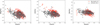 |
Fig. A.1 Comparison between [X/Fe] vs [Fe/H] observed abundance patterns for light elements in the SMC. Orange dots are from Mucciarelli et al. (2023a), whereas grey diamonds are APOGEE DR17 data (Hasselquist et al. 2021). Orange and black contour lines represent density lines of the observed stellar distributions in Mucciarelli et al. (2023a) and Hasselquist et al. (2021), respectively. |
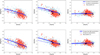 |
Fig. B.1 [X/Fe] vs [Fe/H] for light elements in the SMC adopting different IMFs. Abundance patterns are shown for models adopting a Kroupa et al. (1993) IMF (top panels) and a modified Kroupa et al. (1993) IMF with steeper high-mass end slope (top-light IMF, bottom panels). Solid lines are genuine chemical evolution tracks for models with the re-calibrated SFEs adopted for the particular IMF set-up, while dashed lines are models with the same SFEs used for the reference Kroupa (2001) IMF. Cyan shaded regions are predictions for the model with the re-calibrated SFEs adopted for the IMF set-up, accounting for observational uncertainties ('synthetic model'). Data are as in Fig. 4. |
 |
Fig. C.1 [X/Fe] vs [Fe/H] for n-capture elements for models with increased MNS r-process production at low-metallicity (see Eq. (4)). Solid lines are genuine chemical evolution tracks for the reference models adopting Rubele et al. (2018) SFH (blue) and Massana et al. (2022) SFH (green), whereas shaded cyan and light-green regions are associated model predictions account for observational uncertainties ('synthetic models'). Data are as in Fig. 5. |
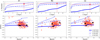 |
Fig. C.2 Mass fraction produced by the s-process channel of production (top panels) and [X/Fe] vs [Fe/H] (bottom panels) for Zr (left panels), Ba (central panels) and La (right panels) for models with different IRV distribution and Kroupa et al. (1993) IMF. Results are shown for models adopting the reference IRV distribution (R150, thick solid lines), R300 distribution (thin dashed), DIS2 distribution (thin dash-dotted) and DIS3 distribution (thin dotted). Data are as in Fig. 8. |
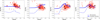 |
Fig. C.3 [X/Fe] vs [Fe/H] for n-capture elements for models with Rubele et al. (2018) SFH, different rate of MNS r-process production at low-metallicity, low-mass AGB yields by Choplin et al. (2022, 2024b), adopting the top-light IMFs defined in 5.2. Blue lines represent models adopting standard (thin dashed) and increased MNS r-process production at low-metallicity (thick solid). Data are as in Fig. 5. |
All Tables
IRV distributions for massive stars (Limongi & Chieffi 2018 models, set R) tested in this study in addition to the reference set (R150; see Sect. 2.3).
All Figures
|
Fig. 1 Global SFHs for the SMC galaxy as derived by Rubele et al. (2018, blue line) and Massana et al. (2022, green line). |
| In the text | |
|
Fig. 2 Age-metallicity relation (top panel) and MDF (bottom panel) as predicted by the reference chemical evolution model adopting Rubele et al. (2018) SFH (blue line, circles and histogram, respectively). The predicted age-metallicity relation is compared with the CMD-extracted relation by Rubele et al. (2018, grey line with confidence intervals), the theoretical curve by Pagel & Tautvaisiene (1998, bursting model, black dashed line), SMC GCs from low-resolution (Parisi et al. 2009, 2015, 2022; Dias et al. 2021, magenta empty circles) and high-resolution studies (Mucciarelli et al. 2023b, red filled squares). Observed MDFs are from Mucciarelli et al. (2023a, red histogram) and Hasselquist et al. (2021, APOGEE DR17, grey histogram). |
| In the text | |
|
Fig. 3 Age-metallicity relation (top panel) and MDF (bottom panel) as predicted by the reference chemical evolution model adopting Massana et al. (2022) SFH (green curve, circles and histogram, respectively). Data are as in Fig. 2. |
| In the text | |
|
Fig. 4 X/Fe] vs [Fe/H] for light elements in the SMC. Abundance patterns are shown for Mg (left panel), Si (central panel) and Ni (right panel) for reference models adopting Rubele et al. (2018) SFH (blue lines and cyan regions) and Massana et al. (2022) SFH (green lines light-green regions). Solid lines are genuine chemical evolution tracks for models with a given SFH, whereas shaded regions are associated model predictions account for observational uncertainties (i.e. synthetic model). Data come from Mucciarelli et al. (2023a, SMC field stars, orange dots) and Mucciarelli et al. (2023b, SMC GCs, black squares). The orange contour lines represent the density lines of the observed stellar distributions in SMC field stars. |
| In the text | |
|
Fig. 5 [X/Fe] vs [Fe/H] for n-capture elements in the SMC. Abundance patterns are shown for Eu (left-most panel), Zr (second left-most) and Ba (second right-most) and La (right-most). Solid lines show the genuine chemical evolution tracks for the reference models adopting Rubele et al. (2018) SFH (blue) and Massana et al. (2022) SFH (green). The shaded cyan and light-green regions are associated model predictions account for observational uncertainties (i.e. synthetic models). Data come from Anoardo et al. (2026, Eu) and Mucciarelli et al. (2023a, Zr, Ba, La) for SMC field stars (orange dots) and Mucciarelli et al. (2023b) for SMC GCs (black dots). The orange contour lines represent density lines of the observed stellar distributions in SMC field stars. |
| In the text | |
|
Fig. 6 [X/Fe] vs [Fe/H] for n-capture elements for the model adopting Rubele et al. (2018) SFH with increased MNS r-process production at low-metallicity (see Eq. (4)). Blue solid lines and cyan shaded regions represent genuine chemical tracks and model predictions accounting for observational uncertainties ('synthetic model'), respectively. Data are as in Fig. 5. |
| In the text | |
|
Fig. 7 [X/Fe] vs [Fe/H] for n-capture elements for the model with Rubele et al. (2018) SFH and increased MNS r-process production at low-metallicity (see Eq. (4)), adopting different IMFs. Blue lines represent models adopting the reference Kroupa (2001) IMF (thin dash-dotted), Kroupa et al. (1993) IMF (thin dashed) and a Kroupa et al. (1993) IMF with steeper high-mass end slope (top-light IMF, thick solid). Cyan shaded regions show the predictions for the model with top-light IMF, accounting for observational uncertainties ('synthetic model'). Data are as in Fig. 5. |
| In the text | |
|
Fig. 8 Mass fraction produced by the s-process channel of production (top panels) and [X/Eu] vs [Fe/H] (bottom panels) for Zr (left panels), Ba (central panels) and La (right panels) for models with different IMFs. In the top panels, we show the results for models adopting the reference Kroupa (2001) IMF (thin dash-dotted lines), Kroupa et al. (1993) IMF (thin dashed), and a modified a top-light IMF (thick solid). In the bottom panels, blue solid lines an cyan shaded regions are genuine chemical tracks and predictions accounting for observational uncertainties ('synthetic model') for a model with a top-light IMF. Data include the Solar s-process mass fraction (Sneden et al. 2008, top panels) and those shown in Fig. 5 (bottom panels). |
| In the text | |
|
Fig. 9 [X/Fe] vs [Fe/H] for Zr, Ba, and La for the model with Rubele et al. (2018) SFH and increased MNS r-process production at low-metallicity (see Eq. (4)), adopting different IRV distributions (see Table 1). Blue lines represent models adopting the reference IRV distribution (R150, thick solid lines), R300 distribution (thin dashed), DIS2 distribution (thin dash-dotted), and DIS3 distribution (thin dotted). Cyan shaded regions are predictions for the model with the DIS2 distribution accounting for observational uncertainties (i.e. synthetic model). Data are as in Fig. 5. |
| In the text | |
|
Fig. 10 Mass fraction produced by the s-process channel of production (top panels) and [X/Eu] vs [Fe/H] (bottom panels) for Zr (left panels), Ba (central panels) and La (right panels) for models with different IRV distributions. In the top panels, we show the results for models adopting the reference IRV distribution (R150, thick solid lines), R300 distribution (thin dashed), DIS2 distribution (thin dash-dotted), and DIS3 distribution (thin dotted). In the bottom panels, blue dash-dotted lines and cyan shaded regions are genuine chemical tracks and predictions accounting for observational uncertainties (i.e. synthetic model) for the model with the DIS2 distribution. Data are as in Fig. 8. |
| In the text | |
|
Fig. 11 [X/Fe] vs [Fe/H] for n-capture elements for the model with Rubele et al. (2018) SFH and low-mass AGB yields by Choplin et al. (2022, 2024b), adopting different IMFs. Blue lines represent models adopting the reference Kroupa (2001) IMF (thin dash-dotted), Kroupa et al. (1993) IMF (thin dashed) and a modified Kroupa et al. (1993) IMF with steeper high-mass end slope (top-light IMF, thick solid). Cyan shaded regions are predictions for the model with top-light IMF accounting for observational uncertainties ('synthetic model'). Data are as in Fig. 5. |
| In the text | |
|
Fig. A.1 Comparison between [X/Fe] vs [Fe/H] observed abundance patterns for light elements in the SMC. Orange dots are from Mucciarelli et al. (2023a), whereas grey diamonds are APOGEE DR17 data (Hasselquist et al. 2021). Orange and black contour lines represent density lines of the observed stellar distributions in Mucciarelli et al. (2023a) and Hasselquist et al. (2021), respectively. |
| In the text | |
|
Fig. B.1 [X/Fe] vs [Fe/H] for light elements in the SMC adopting different IMFs. Abundance patterns are shown for models adopting a Kroupa et al. (1993) IMF (top panels) and a modified Kroupa et al. (1993) IMF with steeper high-mass end slope (top-light IMF, bottom panels). Solid lines are genuine chemical evolution tracks for models with the re-calibrated SFEs adopted for the particular IMF set-up, while dashed lines are models with the same SFEs used for the reference Kroupa (2001) IMF. Cyan shaded regions are predictions for the model with the re-calibrated SFEs adopted for the IMF set-up, accounting for observational uncertainties ('synthetic model'). Data are as in Fig. 4. |
| In the text | |
|
Fig. C.1 [X/Fe] vs [Fe/H] for n-capture elements for models with increased MNS r-process production at low-metallicity (see Eq. (4)). Solid lines are genuine chemical evolution tracks for the reference models adopting Rubele et al. (2018) SFH (blue) and Massana et al. (2022) SFH (green), whereas shaded cyan and light-green regions are associated model predictions account for observational uncertainties ('synthetic models'). Data are as in Fig. 5. |
| In the text | |
|
Fig. C.2 Mass fraction produced by the s-process channel of production (top panels) and [X/Fe] vs [Fe/H] (bottom panels) for Zr (left panels), Ba (central panels) and La (right panels) for models with different IRV distribution and Kroupa et al. (1993) IMF. Results are shown for models adopting the reference IRV distribution (R150, thick solid lines), R300 distribution (thin dashed), DIS2 distribution (thin dash-dotted) and DIS3 distribution (thin dotted). Data are as in Fig. 8. |
| In the text | |
|
Fig. C.3 [X/Fe] vs [Fe/H] for n-capture elements for models with Rubele et al. (2018) SFH, different rate of MNS r-process production at low-metallicity, low-mass AGB yields by Choplin et al. (2022, 2024b), adopting the top-light IMFs defined in 5.2. Blue lines represent models adopting standard (thin dashed) and increased MNS r-process production at low-metallicity (thick solid). Data are as in Fig. 5. |
| In the text | |
Current usage metrics show cumulative count of Article Views (full-text article views including HTML views, PDF and ePub downloads, according to the available data) and Abstracts Views on Vision4Press platform.
Data correspond to usage on the plateform after 2015. The current usage metrics is available 48-96 hours after online publication and is updated daily on week days.
Initial download of the metrics may take a while.