


| Issue |
A&A
Volume 710, June 2026
|
|
|---|---|---|
| Article Number | A267 | |
| Number of page(s) | 16 | |
| Section | Extragalactic astronomy | |
| DOI | https://doi.org/10.1051/0004-6361/202558577 | |
| Published online | 22 June 2026 | |
Short gamma-ray burst progenitors have short delay times
1
STAR Institute, Université de Liège, Sart Tilman, B4000 Liège, Belgium
2
INAF – Osservatorio Astronomico di Brera, via Emilio Bianchi 46, I-23807 Merate (LC), Italy
3
INFN – sezione di Milano-Bicocca, Piazza della Scienza 3, I-20126 Milano (MI), Italy
★ Corresponding author: This email address is being protected from spambots. You need JavaScript enabled to view it.
Received:
15
December
2025
Accepted:
11
May
2026
Abstract
Short gamma-ray bursts (SGRBs) are thought to be primarily associated with binary neutron star (BNS) mergers. The SGRB population can therefore be scrutinized for signatures of the delay time between the formation of the progenitor massive star binary and the eventual merger, which could produce an evolution of the cosmic rate density of such events whose shape departs from that of the cosmic star formation history. We therefore studied a large sample of SGRBs within a hierarchical Bayesian framework, with a particular focus on the delay time distribution (DTD) of the population. Following previous studies, we modelled the DTD either as a power-law with a minimum time delay or as a log-normal function. We considered two models for the intrinsic SGRB luminosity distribution: an empirical luminosity function with a doubly broken power-law shape and another based on a quasi-universal structured jet model. Regardless of the chosen parametrization, we found average time delays of 10 ≲ ⟨τd⟩/Myr ≲ 900 and a minimum delay time of τd, min ≲ 350 Myr, in contrast with previous studies that found long delay times of a few gigayears. We demonstrate that the cause of the longer inferred time delays in past studies most likely resides in an incorrect treatment of selection effects.
Key words: relativistic processes / methods: statistical / circumstellar matter / gamma-ray burst: general
© The Authors 2026
 Open Access article, published by EDP Sciences, under the terms of the Creative Commons Attribution License (https://creativecommons.org/licenses/by/4.0), which permits unrestricted use, distribution, and reproduction in any medium, provided the original work is properly cited.
This article is published in open access under the Subscribe to Open model. This email address is being protected from spambots. You need JavaScript enabled to view it. to support open access publication.
1. Introduction
Gamma-ray bursts (GRBs) are high energy gamma-ray transients of astrophysical origin. They are thought to be produced as a result of cataclysmic astrophysical events, and they are commonly classified according to their time duration and spectral hardness (Kouveliotou et al. 1993; von Kienlin et al. 2020): Short GRBs (SGRBs) are shorter in time duration and on average harder in energy spectrum compared to long GRBs (LGRBs). While a sizeable number of LGRBs have been solidly associated with extreme cases of core-collapse supernovae (CCSNe), SGRBs are believed to mainly be associated with compact binary coalescence (CBC) events, namely binary neutron star (BNS) or neutron star-black hole (NSBH) mergers (Berger 2014). This connection was cemented by the joint observation and unambiguous association of GRB 170817A and the gravitational wave signal GW170817 from a BNS merger (Abbott et al. 2017).
Studies of the SGRB population generally aim to study the intrinsic luminosity distribution (also known as the ‘luminosity function’) of those events, inferring its parameters from a sample of GRBs observed at cosmological distances by various instruments. While some studies describe the luminosity distribution as an empirically defined function (Wanderman & Piran 2015, hereafter W15; Ghirlanda et al. 2016, hereafter G16), others have tested the structured jet hypothesis by utilising more physically motivated models to describe the emitted luminosity (Tan & Yu 2020; Salafia et al. 2023, hereafter S23).
Bearing in mind the CBC origin scenario, the cosmological rate density evolution of the SGRB population depends on the time needed by the compact objects to form from massive stars and for the binary system to merge. Simple theoretical considerations for a BNS system whose orbital separation shrinks due to gravitational radiation suggest that time delays (τd) between the star formation and the merger should be distributed as a power-law dP/dτd ∝ τd−ατ with ατ ∼ 1 (Piran 1992). This model has been widely used in SGRB population studies (e.g. Paul 2018, Tan & Yu 2020, W15). For example, W15, who studied a sample of SGRBs detected by the Fermi Gamma-ray Burst Monitor (Fermi/GBM), the Swift Burst Alert Telescope (Swift/BAT), and the Compton Gamma-Ray Observatory Burst And Transient Source Experiment (CGRO/BATSE), found a delay-time distribution (DTD) power-law index ατ ∼ 1, keeping the minimum time delay fixed at τdmin = 20 Myr. Some works suggest, though, that the power-law index of the DTD might be steeper, leading to shorter coalescence times. D’Avanzo et al. (2014), for example, selected a sample of Swift/BAT using quality cuts that maximise the probability of a redshift measurement and found that its DTD is best represented by ατ ∼ 1.5 and τdmin = 10 Myr. More recent studies of the association between SGRB events with their host galaxies (Zevin et al. 2022) also inferred a steeper power-law DTD, with ατ ∼ 1.5 − 2.2, but with larger minimum time delays, τdmin ∼ 105 − 250 Myr. An analysis of the chemical enrichment of r-process heavy elements in the Milky Way, on the other hand, under the assumption that they are mostly generated in BNS mergers, finds that fast mergers are required, with ατ ≳ 2.0 and τmin ≲ 40 Myr (Chen et al. 2025).
Another widely adopted model of the SGRB DTD is a log-normal distribution ![Mathematical equation: $ \mathrm{d}P/\mathrm{d}\tau_{\mathrm{d}} = \exp[-1/2(\ln\tau_{\mathrm{d}}-\ln\mu_\tau)^2/2\sigma_\tau^2)]/\sigma_\tau\tau_{\mathrm{d}}\sqrt{2\pi} $](/articles/aa/full_html/2026/06/aa58577-25/aa58577-25-eq1.gif) , for which W15 finds μτ ∼ 3 − 4 Gyr and στ ≲ 0.2. Similar values are reported by Luo et al. (2022), where a simulated SGRB population with a structured jet model fitting with the observed Fermi/GBM photon flux distribution is shown to be compatible with a log-normal DTD, disfavouring power-law and Gaussian DTD models.
, for which W15 finds μτ ∼ 3 − 4 Gyr and στ ≲ 0.2. Similar values are reported by Luo et al. (2022), where a simulated SGRB population with a structured jet model fitting with the observed Fermi/GBM photon flux distribution is shown to be compatible with a log-normal DTD, disfavouring power-law and Gaussian DTD models.
Some works find different evolution branches for the BNS population, which can correspond to different BNS formation channels. Studies of BNS systems in our Galaxy show that the BNS population might be composed of two distinct sub-populations: a ‘fast’ population, with either a power-law DTD with ατ ∼ 2 (Maoz & Nakar 2025) or a log-normal one with μτ ∼ 300 Myr and στ ∼ 1 (Beniamini & Piran 2019), and a ‘slow’ population, with τd typically above ∼1 Gyr and with ατ ∼ 1. In particular, Maoz & Nakar (2025) estimates that within Galactic BNS systems that merge within a Hubble time, the fast component is about ten to 100 times more abundant than the slow one. Beniamini & Piran (2019) reached a similar but slightly weaker conclusion that almost half of the Milky Way BNS population must belong to the fast-merging channel. Multi-band optical and near-infrared observations of SGRB host galaxies aimed at measuring their stellar masses and population ages (Leibler & Berger 2010) have shown a similar duality, where long (τd ∼ 3 Gyr) and short time delays (τd ∼ 0.2 Gyr) are respectively associated with early and late-type galaxies.
In this paper we perform a study of the SGRB population, assuming two different models of the DTD and two distinct models of the luminosity function, to test the robustness of our conclusions. The parameters are inferred within a hierarchical Bayesian framework (Mandel et al. 2019, hereafter M19).
In Sect. 2 we describe our methodology and sample selection. Results are shown in Sect. 3 and discussed in Sect. 4, where we also demonstrate a few possible sources of biases, and we analyse their impact on inferring the parameters of our population.
2. Methods
2.1. Bayesian hierarchical inference method
Our approach to characterise the SGRB population closely follows S23, with some updates that we describe below. The parameters of the population model (formally called ‘hyper-parameters’) constitute the elements of the hyper-parameter vector λ′pop. Each SGRB is described by a vector of source parameters, λsrc, i, which are estimated based on the measured data, di (here i = 1, ..., Nobs and Nobs is the number of events in the sample). Following Eqs. 7 and 8 in M19, the posterior probability distribution function (PDF) can be written as
 (1)
(1)
Here π(λpop′) is the ‘hyper-prior’, that is, the joint prior on the hyper-parameters, and P({di}) is the Bayesian evidence of the data (in practice, a normalisation constant). The likelihood of the data given the hyper-parameters, P({di}|λ′pop), is written as a product of single-source terms, each of which is expressed as a ratio of a numerator over a denominator:
 (2)
(2)
and
 (3)
(3)
Here, Ppop(λsrc|λ′pop) is the ‘population probability’ that specifies the probability density of the source parameters for any choice of the hyper-parameters, and Pdet(λsrc) is the selection function. It represents the probability that an event with source parameters λsrc, sampled from the population, is selected and hence included in the sample. The selection function therefore contains all the information on selection effects that stem from both the detection process and from any additional selection cuts that define the sample. Further, P(di|λsrc) is the likelihood of measuring the data for a single event given the source parameters. This framework has been implemented in the publicly available grbpop code1, which we used as a starting point to implement different SGRB population models.
2.2. Including the observed number of events in the inference
To take into account the information on the number of events in the sample and hence include the SGRB local rate density (R0) as one of the parameters of the population, we updated the definition of our posterior probability by embedding the Poissonian probability of the number of observed events. Following Eq. (11) in M19, given the total rate of astrophysical events in a population,
 (4)
(4)
with λpop ≡ (λ′pop, R0), the number of expected detections for a sample of a given detector is
 (5)
(5)
where ηDC is the product of the detector duty cycle times the average fraction of the sky accessible to it,2R(λpop) is the total cosmic rate of events, T is the duration of the observation period, and 𝒟(λ′pop) is the term defined in Eq. (3), which can be shown to be equivalent to the fraction of events in the population that pass the detection and selection cuts. The probability of observing Nobs events given Ndet(λpop) is then a Poissonian probability, and the posterior PDF becomes
![Mathematical equation: $$ \begin{aligned} P(\boldsymbol{\lambda }_\mathrm{pop} |\{\boldsymbol{d}_i\}) = \frac{\pi (\boldsymbol{\lambda }\prime _\mathrm{pop} )}{P(\{\boldsymbol{d}_i\})} \prod ^{N_\mathrm{obs} }_{i = 1} \left[ \frac{\mathcal{N} _i (\boldsymbol{d}_i|\boldsymbol{\lambda }\prime _\mathrm{pop} )}{\mathcal{D} (\boldsymbol{\lambda }\prime _\mathrm{pop} )} \right] e^{-N_\mathrm{det} } (N_\mathrm{det} )^{N_\mathrm{obs} }, \end{aligned} $$](/articles/aa/full_html/2026/06/aa58577-25/aa58577-25-eq7.gif) (6)
(6)
where the  term is omitted due to the distinguishability of the events in the sample (M19). We defined the isotropic equivalent of the peak luminosity, L(p[E0, E1], Ep, z), following Eq. (17) in S23 and modelling the SGRB photon spectrum as a power-law with an exponential cut-off Ghirlanda et al. (2004), with the low-energy photon index set to the median value of α based on the spectral analysis of the Fermi/GBM SGRB catalogue (S23).
2.3. Population models
2.3.1. Rate density evolution
Guided by the expectation that short GRBs are generated mainly in compact binary mergers, such as BNS or NSBH systems, the redshift probability distribution was modelled considering a fixed cosmic star formation history (CSFH) and by convolving it with the distribution of time delays (τd) between the binary system formation and the eventual merger. We considered two DTD models: a power law with a minimum time delay cut-off, namely
 (7)
(7)
where the free parameters are τdmin and the index ατ, and a log-normal DTD, that is
![Mathematical equation: $$ \begin{aligned} P( \tau _\mathrm{d} |\boldsymbol{\lambda }\prime _\mathrm{pop} ) = \exp \left[ - \frac{1}{2} \left( \frac{\ln \tau _\mathrm{d} - \ln \mu _\tau }{\sigma _\tau } \right)^2 \right] (\tau _\mathrm{d} \sqrt{2 \pi \sigma _\tau ^2})^{-1}, \end{aligned} $$](/articles/aa/full_html/2026/06/aa58577-25/aa58577-25-eq10.gif) (8)
(8)
where the parameters to constrain are the median value μτ and the dispersion στ. The rate density distribution is therefore
 (9)
(9)
where ψ(z) is the CSFH and tLB(z) is the cosmological lookback time at redshift z. We chose to adopt the CSFH model from Madau & Fragos (2017),
 (10)
(10)
with aψ = 2.6, bψ = 6.2, and zψ = 2.2. The redshift probability distribution of SGRBs is then computed as
 (11)
(11)
where dV/dz is the differential comoving volume at redshift z.
2.3.2. Luminosity function models: ELF and QUSJ
To describe the luminosity function (i.e. the luminosity PDF) of our population, we chose two different models. The first one, which we refer to as the ‘empirical luminosity function’ model (ELF hereafter), is based on a doubly broken power-law luminosity function, and it extends the W15 luminosity function model to lower luminosities. Following3 Abbott et al. (2022), we express the luminosity function in this model as
 (12)
(12)
Here L0, L**, and L* are the minimum luminosity, low-luminosity break, and high-luminosity break, respectively. The power-law indices of the three branches are expressed through the γBPL, αBPL, and βBPL parameters to facilitate comparison with Abbott et al. (2022). As a way to incorporate some information from GRB 170817A in this model, we chose our prior on L0 to ensure that L0 < L17A, where  is the peak luminosity of GRB 170817A (S23).
To fully specify the population properties, the PDF of the peak photon energy Ep of the GRB spectral energy distribution across the population must also be specified. Following S23, we modelled this as a log-normal distribution with a median value that depends on L:
![Mathematical equation: $$ \begin{aligned} P(E_\mathrm{p} |L, \boldsymbol{\lambda }\prime _\mathrm{pop} ) = \frac{\exp \left[ - \frac{1}{2} \left( \frac{\ln (E_\mathrm{p} ) - \ln (\tilde{E}_\mathrm{p} (L) )}{\sigma _\mathrm{c} } \right)^2 \right]}{E_\mathrm{p} \sqrt{2 \pi \sigma _\mathrm{c} ^2}}, \end{aligned} $$](/articles/aa/full_html/2026/06/aa58577-25/aa58577-25-eq16.gif) (13)
(13)
where  allows for a Yonetoku-like correlation (Yonetoku et al. 2004) when y ≠ 0. The source parameters L and Ep are therefore parametrized with a common probability density: P(L, Ep|λ′pop) = P(Ep|L, λ′pop)P(L|λ′pop).
The second model we considered is the quasi-universal structured jet population model (QUSJ hereafter) from S23, which also features a correlated joint distribution of L and Ep, induced by the jet structure. The latter is defined by two dimensionless functions of the ratio of the viewing angle, θv, to the ‘jet core’ angle θc, written as ℓ(θv/θc) and η(θv/θc), that describe how the luminosity and Ep depend on the jet viewing angle (see S23 for more details). In the analysis based on the QUSJ model, we include the information on the luminosity, peak photon energy, and viewing angle of GRB 170817A in the form of priors on the population parameters, following S23.
In both cases the redshift probability distribution, P(z|λ′pop), is assumed to be independent of L and Ep. The distribution of source parameters across the population is therefore
 (14)
(14)
2.3.3. W15 population model
To gain insight on the difference between our results and those of previous studies, we set out to reproduce the W15 constraints using hierarchical Bayesian inference but with the same sample and selection effects modelling used in that work. For this purpose, the luminosity probability distribution P(L|λ′pop) we employed is the same as in Eq. (12), but we fixed L0 = L** = 5 × 1049 erg s−1. The parameters to be constrained for P(L|λ′pop) therefore are only αBPL, βBPL, and L*.
The redshift probability distribution, P(z|λ′pop), was modelled as in Sect. 2.3.1. The only difference is for the power-law DTD model, where the minimum time delay was fixed to τdmin = 20 Myr. The SGRB photon spectrum dṄ/dE(E,p) was modelled as a Band function Band et al. (1993), whose parameters were fixed to Ep = 800 keV, αBand = −0.5, and βBand = −2.25, as in the original paper (motivated by the analysis of Nava et al. 2011).
Since the spectral energy peak in this model is fixed, the source parameters are only the GRB luminosity and redshift, that is, λsrc = (L, z). In Appendix A we give technical details on how this difference is handled in the inference.
2.4. Samples and detection efficiencies
When building our reference SGRB samples, we needed to carefully model the selection effects that moulded them. We therefore considered two samples for the analysis, built in the same way as in the ‘flux-limited sample analysis’ of S23.
The likelihood numerators, 𝒩i(di|λ′pop), for each event in the samples and denominators, 𝒟(λ′pop), were then computed in the same way as in S23 for both the ELF and the QUSJ case since the only term that changes between the two models is Ppop(λsrc|λ′pop).
2.4.1. Observer-frame sample
The first sample consists of short GRBs detected by Fermi/GBM with publicly available spectral analysis results. We selected events with T90 < 2 s from the GBM’s first 10 years of observation, namely from the 12 July 2008 to 11 July 2018. We applied a completeness cut on the 64 ms peak photon flux in the [50 − 300] keV energy band, selecting only the events with p[50, 300] > plim, GBM = 3.50 cm−2 s−1, which is the value above which we can consider our sample as complete in flux (S23). Additional cuts on the observed spectral peak energy (Ep, obs) were applied, considering only events with best-fit values 50 keV ≤ Ep, obs ≤ 10 MeV, which is the spectral range where the effective area of the Fermi/GBM detectors is optimal. After all cuts, the sample contained 210 short GRB events. Hereon, we refer to this as the ‘observer-frame sample’.
The detection efficiency for this sample was modelled as
![Mathematical equation: $$ \begin{aligned}&P_{\mathrm{det} }(L, E_\mathrm{p} ,z) = \Theta \left(p_{[50, 300]}(L,E_\mathrm{p} ,z) - p_\mathrm{lim,GBM} \right)\times \nonumber \\&\quad \Theta \left(E_\mathrm{p} /(1+z)-50\,\mathrm{keV} \right)\Theta \left(10\,\mathrm{MeV} -E_\mathrm{p} /(1+z)\right), \end{aligned} $$](/articles/aa/full_html/2026/06/aa58577-25/aa58577-25-eq19.gif) (15)
(15)
where Θ(x) is the Heaviside step function.
Given the number of events contained in the observer-frame sample, we considered its event detection rate to estimate the astrophysical local rate density (R0) of the SGRB population. The Ndet for the Poissonian term in Eq. (6) was therefore computed using the 𝒟(λ′pop) for this sample, an observation period of T = 10 yr, and a multiplicative factor of ηDC = 0.59 accounting for both the accessible field of view and the duty cycle of Fermi/GBM (Burns et al. 2016).
2.4.2. Rest-frame sample
The second sample consist of short GRBs detected by Fermi/GBM and Swift/BAT that pass a set of stringent cuts that maximise the redshift completeness without distorting the redshift distribution. In practice, this is the sub-sample of the S-BAT4ext catalogue (Ferro et al. 2023) of events that were also detected by Fermi/GBM. The selection includes a Swift/BAT completeness flux threshold in the [15 − 150] keV energy band, p[15, 150] > plim, BAT = 3.50 cm−2 s−1, in addition to the same Fermi/GBM completeness cuts as in the observer-frame sample. The sample consists of 18 short GRBs events, 16 of which have a measured redshift. For those events we used the results of the spectral analysis performed in S23, which yields, for each event i, a posterior on the source parameters P(L, Ep, z | di), given a prior π(L, Ep, z)∝(1 + z)−1L−1. We refer to this sample as the ‘rest-frame sample’. We did not use the number of events in this sample to inform our estimate of R0 because of the difficulty in correctly modelling the duty cycle factor ηDC incorporating all the cuts that define the sample.
Because we required the detection by Fermi/GBM, the rest-frame sample detection efficiency includes the same cuts as the observer-frame sample. In addition, it features a factor
![Mathematical equation: $$ \begin{aligned} \Theta \left(p_{[15, 150]}(L,E_\mathrm{p} ,z) - p_\mathrm{lim,BAT} \right) \end{aligned} $$](/articles/aa/full_html/2026/06/aa58577-25/aa58577-25-eq20.gif) (16)
(16)
to account for the Swift/BAT completeness cut. All other S-BAT4 cuts are independent on the source properties and hence do not enter the definition of this efficiency.
We note that GRB 170817A is not included in either of the two samples because its peak flux is below the Fermi/GBM completeness threshold. In the case of the quasi-universal jet population model, our results still include information on this event in the form of a prior on the hyper-parameters, which we built following the procedure used by S23 in their flux-limited sample analysis.
2.4.3. W15 samples
The observer-frame samples considered for the W15 population analysis consist of short GRBs observed by Fermi/GBM, CGRO/BATSE, and Swift/BAT. For the three detectors, the detection efficiency was modelled as a hard threshold on the 64 ms peak photon flux in their respective most sensitive detector energy band, as in Eq. (16). The photon flux thresholds considered for CGRO/BATSE and Fermi/GBM in the [E0, E1]=[50, 300] keV detector energy band for this analysis were, respectively, plim, BATSE = 1.5 cm−2 s−1 and plim, GBM = 2.37 cm−2 s−1, while for Swift/BAT it was plim, BAT = 2.5 cm−2 s−1 in the [E0d, E1d]=[15, 150] keV band.
The BATSE and Fermi sample contain GRBs with a measured p[E0, E1] above the respective detector threshold and T90 < 2 s. While for BATSE these selection effects have been applied to the entirety of its catalogue, for a total of 414 events, the Fermi/GBM events were considered up to the 10 April 2013, as in W15, yielding 146 bursts.
The rest-frame sample was built following W15. The sample contains events detected by Swift/BAT with a measured redshift and L, with T90 < 2 s, up to GRB 131004A. A cut on the probability of having a non-collapsar origin higher than 60%, estimated following Bromberg et al. (2013), was then applied, selecting a sub-sample of 12 events.
Since the spectral peak energy in this analysis is fixed to a punctual value in the source frame, the computation of the likelihood was a bit different from that in the ELF and QUSJ cases. Full details on the likelihood evaluation and the obtained results are described in Appendix A. In the following, we refer to the results of this analysis as W15*.
2.5. Priors and posterior evaluation
We chose broad priors on most parameters, considering either a uniform or a uniform-in-log distribution within a defined range for each parameter, with the following exceptions: (i) For θc and θw, we considered an isotropic prior (i.e. uniform in the subtended solid angle) π(θc/w)∝sin(θc/w). (ii) For the minimum luminosity of the ELF model, we chose the upper bound of the prior based on the luminosity of GRB 170817A, as stated previously. (iii) For the QUSJ model, we followed the approach of S23 to condition the prior on the observed properties of GRB 170817A (see their section 2.5.3). The bounds that we report in Table 1 refer to the priors before that conditioning. The population parameters were considered to be independent from each other, with the exceptions of (L0, L**, L*) for the ELF model and (θc, θw) for the QUSJ model. In fact, for the triplet of luminosity breaks, we imposed L0 < L** < 1051 erg s−1 < L*, while for the break angles in the quasi-universal jet structure, we set θc < θw. The choice to put a boundary between L** and L* at L = 1051 erg s−1 was motivated by wanting to avoid that those parameters have local peaks in the posteriors in the same parameter region. Common parameters in the two population models share common priors. The full set of priors for each parameter with their bounds are shown in Table 1.
Full set of population parameters and the associated priors.
The posterior PDF was estimated through dynamical nested sampling using the open source python package dynesty (Higson et al. 2019); dynesty. The number of initial live points was set to 100 times the dimensionality of the posterior PDF, for a total of 1200 and 1400 initial live points, respectively, for the ELF and the QUSJ models. As stopping criteria, we chose dlogz = 10−5 and 30 000 effective samples. Batches of live points were periodically and automatically added to reach those criteria, with each batch containing one fifth of the initial live points used for the sampling. The obtained posterior PDFs for all the cases considered are portrayed as corner plots in Appendix B, with contours representing the 90% and 50% confidence levels, while the estimated median values of the parameters with their 90% credible intervals are shown in Table 2.
Constraints on population parameters.
3. Results
A summary of the constraints obtained on the population parameters for the ELF and QUSJ models, with both the power-law and log-normal DTDs, is given in Table 2. The results for the W15* analysis are reported in Appendix A, where we demonstrate a good agreement with the results in the original paper.
3.1. Time delay and redshift distribution
We illustrate the constraints obtained with our analyses on the shape of the rate density evolution with redshift in Fig. 1 (left-hand panels), where the  curves (i.e. the SGRB rate density normalised to its value at z = 0) are compared with the normalized CSFH. The results are quite consistent between the ELF and QUSJ models, where the curves tend to closely follow the CSFH, while the W15* analysis yields a very different constraint. The DTD parameter constraints (right-hand panels) show that this is the result of much shorter time delays in our models with respect to those obtained in the W15* analysis. To make this more evident and to enable a comparison between different DTD models, we also show in the figure, in addition to the posterior probability on the DTD parameters, the distribution of the average time delay:
 (17)
(17)
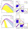 |
Fig. 1. Rate density distributions as functions of redshift (left panels) and corner plots of the posterior PDFs for the DTD parameters and ⟨τd⟩ (right panels). Top and bottom panels show the results obtained with a power-law and a log-normal DTD, respectively. Rate density distributions are normalised to 1 at z = 0, and the CSFH from Madau & Fragos (2017) is shown in purple for comparison. Red and blue curves represent the distributions obtained considering, respectively, the ELF and the QUSJ models. W15* results are displayed in yellow. |
In the power-law DTD scenario, both luminosity function models show a steep power-law index ατ > 1.5, while the minimum time delays are below τd < 370 Myr (90% credible limits). The average time delays are generally below ∼1 Gyr, with a median and 90% credible range of  (ELF) or
  (QUSJ). The time delays associated with the W15* DTD parameters, on the other hand, were found to be significantly larger, yielding
  .
.
Similar results were obtained in the log-normal DTD case, where the median value of the log-normal distribution is μτ < 700 Myr, while σc is only loosely constrained to be somewhat below the upper end of its prior range, which is equivalent to 1.5 dex. For the ELF and QUSJ models, the average time delays are respectively  and
and  , while the W15* analysis yields
  .
.
3.2. Luminosity function
The red (resp. blue) filled areas in Figure 2 show the 90% credible bands of the luminosity function obtained assuming the ELF (resp. QUSJ) model for the power-law DTD (left-hand panel) and the log-normal DTD (right-hand panel). In each panel, we also show the corresponding result of the W15* analysis. The luminosity of GRB 170817A (S23) is shown with a vertical grey band for comparison.
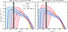 |
Fig. 2. Luminosity probability distributions obtained considering either a power-law or a log-normal DTD (left and right panel, respectively). Results obtained with the broken power-law model are shown in red, and the ones obtained with the structured jet model are in blue. The shaded areas represent the 90% credible intervals. Luminosity functions from W15 are also shown in yellow. The measured luminosity for GRB 170817A is shown in grey as a reference point. |
The two different DTD models considered have a limited impact on the shape of the luminosity function. Above Liso ∼ 5 × 1052 erg s−1, both of our luminosity function models show good agreement with each other and with the W15* results. Between Liso ∼ 1049 erg s−1 and Liso ∼ 1052 erg s−1, the trend of the ELF tends to follow the one from W15*, while the structured jet model curves have a slightly shallower slope. This is a result of the choice of parametrization and a consequence of the larger amount of information on GRB 170817A included in the QUSJ model. Below Liso ∼ 1049 erg s−1, the ELF model shows very large rate uncertainties compared to the structured jet scenario. This is again a consequence of the information from GRB 170817A included in that model, and in part it also reflects the stronger predictivity of the QUSJ model at low luminosity, where the minimum luminosity is set by the maximum possible viewing angle and by the slope of the apparent structure.
3.3. Local rate density
As shown in Fig. 3, the overall local rate density inferred using the ELF has a larger uncertainty compared to the result using the QUSJ model, regardless of the chosen DTD model. This is a direct consequence of the reduced predictivity of the ELF model on the minimum SGRB luminosity compared to the QUSJ model. It is instructive to compare these rate density constraints with the most recent local BNS merger rate density constraint inferred from gravitational wave observations, based on the fourth gravitational wave transient catalogue (GWTC-4; Abac et al. 2025, R0 ∈ [7.6, 250] Gpc−3 yr−1 as shown by the vertical grey band in the figure). For the ELF model with the power-law DTD and the QUSJ model with the log-normal DTD, most of the posterior support is within the GWTC-4 BNS rate density constraint. For the QUSJ model with the power-law DTD, the support is concentrated at somewhat higher local rate densities, but a substantial fraction of the probability is still within the gravitational wave constraint. The ELF model with the power-law DTD rate posterior peaks within the GWTC-4 BNS rate density boundaries, reaching almost a plateau up to the upper prior PDF bound. This is a result of the poor constraints on the L** parameter in this case, which is correlated with log R0 (see Fig. B.3 in Appendix B). In general, these results support a scenario where BNS mergers constitute the progenitors of the vast majority of SGRBs, in line with the conclusions of S23.
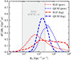 |
Fig. 3. Comparisons between local rate density probability distributions. Distributions obtained with the broken power-law and the structured jet luminosity models are shown in red and blue, respectively, while results corresponding to power-law and log-normal DTD are respectively displayed with dashed and dotted lines. The BNS rate density inferred from gravitational wave observations (Abac et al. 2025) is shown in grey (90% credible intervals). |
4. Discussion
The estimated time delays based on all four combinations of the models considered range between ∼11 − 18 Myr and ∼764 − 854 Myr. The lower end of these distributions can be explained by fast BNS merger channels, which may happen in binary star systems forming with a short orbital separation and evolving quickly through a common envelope and a mass transfer phase (Tauris et al. 2017), where the merger time can further decrease thanks to neutron star natal kicks (Andrews & Zezas 2019; Beniamini & Piran 2024). The parameter ranges found for the power-law DTD are compatible with those estimated from the Milky Way r-process element abundances (Chen et al. 2025), suggesting that BNS mergers are responsible for a significant fraction of those elements in our Galaxy.
Nonetheless, our findings for both DTD models contrast with time delay estimations in other short GRB population studies, such as W15, Luo et al. (2022) and Tan & Yu (2020). The differences could in part be traced back to the different SGRB samples with a measured redshift considered. For example, the largest measured redshift for a GRB of the W15 sample is z = 1.131, while our sample contains four GRBs with a measured redshift beyond that value, up to z = 2.28 ± 0.14.
However, the different treatment of the selection effects could also play a role in the estimate of the SGRB time delays. On one hand, the chosen peak-flux thresholds for Fermi/GBM in W15 and Tan & Yu (2020) and for Swift/BAT in W15 are below the respective completeness flux thresholds. Moreover, many previous studies relied on rest-frame samples (i.e. samples of GRBs with measured redshifts) constructed without a careful assessment of their selection effects and how these could have distorted their redshift distribution. To test for the impact of incorrectly modelling the selection effects on inferring the time delay parameters, we performed the additional analysis runs described below.
To demonstrate the biases deriving from using a flux-incomplete sample, we simulated a sample of short GRBs with an ELF and a power-law DTD using the following parameters: αBPL = 2, βBPL = 3, γBPL = 1, L0 = 1046 erg s−1, L** = 1048 erg s−1, L* = 1052 erg s−1, τdmin = 0.1 Myr, ατ = 1, Ep★ = 1 MeV, y = 0.3, and σc = 1. We considered Fermi/GBM as the only detector, and we modelled its detection efficiency following S23. Figure 4 shows the assumed detection efficiency as a function of p[50, 300] (black line; in the plot we assume Ep, obs = 100 keV, but the dependence on the latter parameter is weak; see S23). This allowed us to obtain a sample of 271 simulated SGRBs that were ‘detected’. We divided this sample into an observer-frame and a rest-frame sample of 241 and 30 events, respectively. For the inference runs, we considered a hard flux threshold detection efficiency model Pdet(L, Ep, z) = Θ(p[50, 300](L,Ep,z)−plim) for different values of plim, namely 3.5, 3.0, 2.5, and 1.5 cm−2 s−1 (the assumed detection efficiency models are shown by the thick coloured lines in Fig. 4). For each plim value considered, we ran the inference method only on the sub-sample of simulated SGRBs brighter than that threshold.
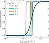 |
Fig. 4. Comparison between the detection efficiency in our simulated sample and that used in the inference. The solid black line shows the detection efficiency model pdet, GBM from S23 as a function of the SGRB photon flux, assuming Ep, obs = 100 keV. The thick coloured lines show the hard-threshold detection efficiency models assumed in our inference of the simulated sample described in Sect. 4, with different colours indicating different assumed photon flux thresholds, as in Figure 5. For each of these analyses, only the SGRBs above the assumed threshold were included in the inference. |
Figure 5 shows the posterior distribution of the average time delay for each of these four inference runs. When plim = plim, GBM = 3.5 cm−2 s−1, the sample is ‘complete’ in flux (in practice, the detection efficiency is ≳80% above the chosen threshold), and the posterior distribution peak coincides with the true value of the simulated population ⟨τdtrue⟩ = 2.78 Gyr. When the assumed plim is less than the value of plim, GBM, the inference method systematically overestimates the inferred time delays. This simple simulation shows that the long time delays inferred in previous SGRB population studies might be, at least in part, the result of a bias due to an incorrect modelling of the selection effects.
 |
Fig. 5. Posterior distribution of the average time delays inferred from a simulated SGRB population while assuming different photon peak flux cuts. The dashed black line shows the ‘true’ average time delay value corresponding to the power-law DTD parameters from which the SGRB events have been sampled. The blue curve shows the result obtained with the same flux threshold cut as in our analysis, which ensures flux completeness of the sample. The yellow, green, and pink curves were obtained with lower threshold values, as reported in the legend. |
5. Conclusions
We have performed a hierarchical Bayesian study of the short GRB population in order to determine the time delays between those events and the CSFH. To minimise observational biases, we selected both a flux-complete and a high redshift-completeness sample of SGRBs. We considered two different models for the delay time distribution, namely, a power-law with a minimum time delay and a log-normal distribution, and we modelled the luminosity probability distribution of our population either as a doubly broken power law or starting from a quasi-universal jet structure. We chose the CSFH from Madau & Fragos (2017).
The inferred parameters for a power-law delay time distribution model are compatible with the estimates from the r-process elements in our Galaxy (Chen et al. 2025), and they correspond to time delays ranging from ∼12 Myr to ∼686 − 770 Myr. The steep power-index (ατ > 1.5) deviates from the ‘conventional’ value ατ = 1 adopted for a binary system that evolves while losing energy solely through gravitational radiation. This suggests that compact binary systems can merge through faster channels, for example forming with a low initial orbital separation and undergoing through a common envelope and mass transfer phase (Tauris et al. 2017). In some cases, the time required by the binary to merge might further reduce when neutron star natal kicks occur (Andrews & Zezas 2019; Beniamini & Piran 2024). The same fast merger channel scenarios are compatible with our findings for a log-normal delay time distribution, where the expected time delays go from ∼13 − 14 Myr to ∼877 − 969 Myr.
For each of the delay time distributions considered, we found that the choice of luminosity function model has a limited impact on the time delay results, supporting the conclusion that our finding does not depend specifically on our parametrization of the luminosity function.
Finally, we tested the impact of ill-modelled selection effects on the inferred time delays of a SGRB population by repeating the study for a simulated sample and using different values for its flux cut. We found that the inferred time delays become shifted towards higher values when using a flux threshold lower than the completeness one. We therefore stress the importance of building samples whose selection effects are understood and correctly modelled when performing statistical inference for parameter estimation, in order to minimise the observational biases when studying a population of astrophysical events.
Acknowledgments
MP acknowledges the fundings from the Fonds de la Recherche Scientifique – FNRS, Belgium, under grant No. 4.4501. OS acknowledges support from the Italian National Institute for Astrophysics (INAF) through ‘Finanziamento per la ricerca fondamentale’ grant number 1.05.23.04.04, and also funding by the European Union-Next Generation EU, PRIN 2022 RFF M4C21.1 (202298J7KT – PEACE).
References
- Abac, A. G., Abouelfettouh, I., Acernese, F., et al. 2025, arXiv e-prints [arXiv:2508.18083] [Google Scholar]
- Abbott, B. P., Abbott, R., Abbott, T. D., et al. 2017, ApJ, 848, L13 [CrossRef] [Google Scholar]
- Abbott, R., Abbott, T. D., Acernese, F., et al. 2022, ApJ, 928, 186 [NASA ADS] [CrossRef] [Google Scholar]
- Andrews, J. J., & Zezas, A. 2019, MNRAS, 486, 3213 [NASA ADS] [CrossRef] [Google Scholar]
- Band, D., Matteson, J., Ford, L., et al. 1993, ApJ, 413, 281 [Google Scholar]
- Beniamini, P., & Piran, T. 2019, MNRAS, 487, 4847 [CrossRef] [Google Scholar]
- Beniamini, P., & Piran, T. 2024, ApJ, 966, 17 [NASA ADS] [CrossRef] [Google Scholar]
- Berger, E. 2014, ARA&A, 52, 43 [CrossRef] [Google Scholar]
- Bromberg, O., Nakar, E., Piran, T., & Sari, R. 2013, ApJ, 764, 179 [NASA ADS] [CrossRef] [Google Scholar]
- Burns, E., Connaughton, V., Zhang, B.-B., et al. 2016, ApJ, 818, 110 [NASA ADS] [CrossRef] [Google Scholar]
- Chen, H.-Y., Landry, P., Read, J. S., & Siegel, D. M. 2025, ApJ, 985, 154 [Google Scholar]
- D’Avanzo, P., Salvaterra, R., Bernardini, M. G., et al. 2014, MNRAS, 442, 2342 [Google Scholar]
- Ferro, M., Brivio, R., D’Avanzo, P., et al. 2023, A&A, 678, A142 [NASA ADS] [CrossRef] [EDP Sciences] [Google Scholar]
- Ghirlanda, G., Ghisellini, G., & Celotti, A. 2004, A&A, 422, L55 [NASA ADS] [CrossRef] [EDP Sciences] [Google Scholar]
- Ghirlanda, G., Salafia, O. S., Pescalli, A., et al. 2016, A&A, 594, A84 [NASA ADS] [CrossRef] [EDP Sciences] [Google Scholar]
- Higson, E., Handley, W., Hobson, M., & Lasenby, A. 2019, Stat. Comput., 29, 891 [Google Scholar]
- Kouveliotou, C., Meegan, C. A., Fishman, G. J., et al. 1993, ApJ, 413, L101 [NASA ADS] [CrossRef] [Google Scholar]
- Leibler, C. N., & Berger, E. 2010, ApJ, 725, 1202 [NASA ADS] [CrossRef] [Google Scholar]
- Luo, J.-W., Li, Y., Ai, S., Gao, H., & Zhang, B. 2022, MNRAS, 516, 1654 [NASA ADS] [CrossRef] [Google Scholar]
- Madau, P., & Fragos, T. 2017, ApJ, 840, 39 [Google Scholar]
- Mandel, I., Farr, W. M., & Gair, J. R. 2019, MNRAS, 486, 1086 [Google Scholar]
- Maoz, D., & Nakar, E. 2025, ApJ, 982, 179 [Google Scholar]
- Nava, L., Ghirlanda, G., Ghisellini, G., & Celotti, A. 2011, A&A, 530, A21 [NASA ADS] [CrossRef] [EDP Sciences] [Google Scholar]
- Paul, D. 2018, MNRAS, 477, 4275 [NASA ADS] [CrossRef] [Google Scholar]
- Piran, T. 1992, ApJ, 389, L45 [Google Scholar]
- Planck Collaboration XXX. 2014, A&A, 571, A30 [NASA ADS] [CrossRef] [EDP Sciences] [Google Scholar]
- Salafia, O. S., Ravasio, M. E., Ghirlanda, G., & Mandel, I. 2023, A&A, 680, A45 [NASA ADS] [CrossRef] [EDP Sciences] [Google Scholar]
- Speagle, J. S. 2020, MNRAS, 493, 3132 [Google Scholar]
- Tan, W.-W., & Yu, Y.-W. 2020, ApJ, 902, 83 [NASA ADS] [CrossRef] [Google Scholar]
- Tauris, T. M., Kramer, M., Freire, P. C. C., et al. 2017, ApJ, 846, 170 [Google Scholar]
- von Kienlin, A., Meegan, C. A., Paciesas, W. S., et al. 2020, ApJ, 893, 46 [Google Scholar]
- Wanderman, D., & Piran, T. 2015, MNRAS, 448, 3026 [NASA ADS] [CrossRef] [Google Scholar]
- Yonetoku, D., Murakami, T., Nakamura, T., et al. 2004, ApJ, 609, 935 [Google Scholar]
- Zevin, M., Nugent, A. E., Adhikari, S., et al. 2022, ApJ, 940, L18 [NASA ADS] [CrossRef] [Google Scholar]
The term ηDC in general expresses the fraction of events that pass any pre-selection that does not depend on the properties of the source and is not accounted for in the Pdet selection effects model.
We note that the formulation in Abbott et al. (2022), which is inspired by W15, is in terms of the probability density of the logarithm of the luminosity, dP/dlnL, while in our formalism the quantity P(L | λ′pop) is a probability density of the luminosity, dP/dL. For that reason, the power-law slopes in our formulation are steeper by one with respect to their definition.
Appendix A: Likelihoods and results for W15*
A.1. Likelihood evaluation
The likelihood numerator described in Eq. 2 for the Fermi/GBM and CGRO/BATSE samples are computed in a similar way to what done in S23 but considering the photon spectral peak energy in the source frame fixed to Ep* = 800 keV. We can, in fact, write the posterior probability on the source parameters such as P(λsrc|di) = P(di|λsrc)π(L)π(z)/P(di). Then, assuming that P(λsrc|di)∝π(z) and neglecting the uncertainty on the measured p[E0, E1], we can write
 (A.1)
(A.1)
where  . We can compute the prior on L by assuming a uniform prior in p[E0, E1] and applying a coordinate transform
 (A.2)
(A.2)
so that the numerator for the likelihood terms in the product for each event of the sample we obtain is
 (A.3)
(A.3)
The likelihood numerator for the Swift/BAT sample is built in an analogous way. By neglecting the uncertainty on the measured luminosity and redshift, we have
 (A.4)
(A.4)
If we assume a prior uniform in ln(L) and z, we have that π(L, z)∝L−1, and therefore the likelihood numerator for Swift/BAT events is
 (A.5)
(A.5)
For the events in the three samples, the likelihood denominator can be computed as in Eq. 3:
![Mathematical equation: $$ \begin{aligned} \mathcal{D} (\boldsymbol{\lambda }^\prime _\mathrm{pop} ) = \int \Theta (p_{[E_0, E_1]}(\boldsymbol{\lambda }_\mathrm{src} ,E^*_\mathrm{p} ) - p_{\mathrm{lim} ,k}) P_\mathrm{pop} (\boldsymbol{\lambda }_\mathrm{src} |\boldsymbol{\lambda }^\prime _\mathrm{pop} )\mathrm{d} \boldsymbol{\lambda }_\mathrm{src} \ . \end{aligned} $$](/articles/aa/full_html/2026/06/aa58577-25/aa58577-25-eq99.gif) (A.6)
(A.6)
The astrophysical SGRB local rate density R0 is estimated using the rate of observed SGRBs in the Fermi/GBM sample, with its corresponding 𝒟(λ′pop) and considering an effective observing time of T ⋅ ηDC = 3.65 yr (W15).
A.2. Priors and posterior evaluation
The prior PDFs for the population parameters λ′pop have been chosen independent between each other, i.e. π(λ′pop) = π(αBPL)π(βBPL)π(L*)π(αt)π(R0) and π(λ′pop) = π(αBPL)π(βBPL)π(L*)π(μt)π(σt)π(R0) respectively for the power-law and the log-normal DTD models. All the priors have been chosen either uniform or uniform in logarithm, within the bounds that we can deduce from W15 plots. The set of priors used is listed in table A.1.
Population parameters for the W15 study and priors used in our test.
As in Sect. 2.5, the evaluation of the posterior PDF is performed through dynamical nested sampling. The number of initial live points is set to 200 times the dimensionality of the posterior PDF, for a total of 1000 and 1200 initial live points respectively for the power-law and the log-normal DTD models. As stopping criteria, we choose dlogz = 10−5 and 30000 effective samples and batches of live points were periodically and automatically added to reach those criteria, with each batch containing one fifth of the initial live points.
A.3. Results
The obtained posterior PDF corner plots are shown in Fig. B.1 and Table A.2 shows the values estimated for the parameters of the population. Although the CSFH we used to reproduce those results (Madau & Fragos 2017) is not featured in the W15 study, its trend is very similar to the one from Planck Collaboration XXX (2014), which is one of the models used for the analysis in W15 and referred to as SFR2. We therefore take into account this set of results from W15 to compare ours. The uncertainty taken into account on the median values is 1σ as in W15, in order to make a direct comparison between the two works.
Constraints on parameters for the W15 sample and model. Error bars depict 1σ posterior credible intervals as in W15 to make a direct comparison between the parameters inferred.
The results are quite similar to those of W15, except for a shorter median time delay and a larger variance for the log-normal DTD and the local rate density whose estimate is one order of magnitude higher than the one in W15. We attribute the difference in the estimate of R0 to the different methods used, as in W15 they build their estimate on the fraction of non-collapsar events based on the criteria by Bromberg et al. (2013).
If we perform the same analysis with a wider range of parameters for our prior PDFs, we obtain considerably different results. In fact, if we consider a uniform prior in the interval [ − 3, 5] for αBPL and a uniform-in-log prior for L* between [1050, 1054] erg s−1, the posterior starts to exhibit multiple local maxima as shown in Fig. B.1.
By looking at the luminosity functions obtained with these extended prior bounds (Fig. A.1), we can see that both in the power-law and the log-normal case they peak around Liso ∼ 2 × 1050 erg s−1, following a single power-law trend after.
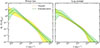 |
Fig. A.1. Luminosity functions obtained with the sample and model from W15, obtained considering a power-law and a log-normal DTD (respectively left and right panel). The yellow dashed curves correspond to the original parameter range considered for the study, while the green continuous curves represent the results obtained with a wider parameter range. Shaded areas depict the 90% percentiles. |
The redshift distributions obtained, displayed in Fig. A.2, present different behaviours for the two delay time distribution models. The power-law model with fixed minimum time delay brings to a considerable uncertainty in the peak of the distribution, ranging from z ∼ 0 to z ∼ 2 when considering a 90% credible interval. Overall the curves look a bit shifted towards lower redshift when compared to the ones obtained with the tighter parameter range. On the other hand, the curves obtained with the log-normal model and a wider parameter range have a similar behaviour to what has been found in W15, but with a larger uncertainty on the distribution. The larger credible intervals are related to the wider log στ values found with the choice of a less restrictive prior for the other parameters (see Fig. B.1).
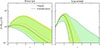 |
Fig. A.2. Redshift distribution of SGRBs for the W15* population normalised to 1 at z = 0. The power-law and log-normal DTD scenarios are shown, respectively, in the left and right panel. The yellow dashed curves depict the original parameter range considered for the study, while the green continuous curves show the results obtained with a wider parameter range. Shaded areas correspond to the 90% percentiles. |
Appendix B: Posterior PDF corner plots
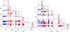 |
Fig. B.1. Posterior PDF contour plots for the W15* results along with the marginalised posterior PDFs on the sides for each parameter, in the power-law DTD (left panel) and log-normal DTD (right panel) cases. Red and blue contours respectively represent the results obtained using the "original" and extended priors on the parameters. Darker and lighter shades of the contours depict, respectively, the 50% and 90% confidence levels. The error bars on the marginalised posteriors mark the median of the parameters along with their 1 σ uncertainty. |
 |
Fig. B.2. Corner plot of the posterior PDF for the ELF + power-law DTD model, with the relative marginalised posteriors for each parameter. Contours depict the 50% and 90% confidence levels. Vertical dashed lines on the marginalised posteriors represent the median values with the 90% credible intervals. |
 |
Fig. B.3. Corner plot of the posterior PDF for the ELF + log-normal DTD model, with the relative marginalised posteriors for each parameter. Contours depict the 50% and 90% confidence levels. Vertical dashed lines on the marginalised posteriors represent the median values with the 90% credible intervals. |
 |
Fig. B.4. Corner plot of the posterior PDF for the QUSJ + power-law DTD model, with the relative marginalised posteriors for each parameter. Contours depict the 50% and 90% confidence levels. Vertical dashed lines on the marginalised posteriors represent the median values with the 90% credible intervals. |
 |
Fig. B.5. Corner plot of the posterior PDF for the QUSJ + log-normal DTD model, with the relative marginalised posteriors for each parameter. Contours depict the 50% and 90% confidence levels. Vertical dashed lines on the marginalised posteriors represent the median values with the 90% credible intervals. |
All Tables
Constraints on parameters for the W15 sample and model. Error bars depict 1σ posterior credible intervals as in W15 to make a direct comparison between the parameters inferred.
All Figures
|
Fig. 1. Rate density distributions as functions of redshift (left panels) and corner plots of the posterior PDFs for the DTD parameters and ⟨τd⟩ (right panels). Top and bottom panels show the results obtained with a power-law and a log-normal DTD, respectively. Rate density distributions are normalised to 1 at z = 0, and the CSFH from Madau & Fragos (2017) is shown in purple for comparison. Red and blue curves represent the distributions obtained considering, respectively, the ELF and the QUSJ models. W15* results are displayed in yellow. |
| In the text | |
|
Fig. 2. Luminosity probability distributions obtained considering either a power-law or a log-normal DTD (left and right panel, respectively). Results obtained with the broken power-law model are shown in red, and the ones obtained with the structured jet model are in blue. The shaded areas represent the 90% credible intervals. Luminosity functions from W15 are also shown in yellow. The measured luminosity for GRB 170817A is shown in grey as a reference point. |
| In the text | |
|
Fig. 3. Comparisons between local rate density probability distributions. Distributions obtained with the broken power-law and the structured jet luminosity models are shown in red and blue, respectively, while results corresponding to power-law and log-normal DTD are respectively displayed with dashed and dotted lines. The BNS rate density inferred from gravitational wave observations (Abac et al. 2025) is shown in grey (90% credible intervals). |
| In the text | |
|
Fig. 4. Comparison between the detection efficiency in our simulated sample and that used in the inference. The solid black line shows the detection efficiency model pdet, GBM from S23 as a function of the SGRB photon flux, assuming Ep, obs = 100 keV. The thick coloured lines show the hard-threshold detection efficiency models assumed in our inference of the simulated sample described in Sect. 4, with different colours indicating different assumed photon flux thresholds, as in Figure 5. For each of these analyses, only the SGRBs above the assumed threshold were included in the inference. |
| In the text | |
|
Fig. 5. Posterior distribution of the average time delays inferred from a simulated SGRB population while assuming different photon peak flux cuts. The dashed black line shows the ‘true’ average time delay value corresponding to the power-law DTD parameters from which the SGRB events have been sampled. The blue curve shows the result obtained with the same flux threshold cut as in our analysis, which ensures flux completeness of the sample. The yellow, green, and pink curves were obtained with lower threshold values, as reported in the legend. |
| In the text | |
|
Fig. A.1. Luminosity functions obtained with the sample and model from W15, obtained considering a power-law and a log-normal DTD (respectively left and right panel). The yellow dashed curves correspond to the original parameter range considered for the study, while the green continuous curves represent the results obtained with a wider parameter range. Shaded areas depict the 90% percentiles. |
| In the text | |
|
Fig. A.2. Redshift distribution of SGRBs for the W15* population normalised to 1 at z = 0. The power-law and log-normal DTD scenarios are shown, respectively, in the left and right panel. The yellow dashed curves depict the original parameter range considered for the study, while the green continuous curves show the results obtained with a wider parameter range. Shaded areas correspond to the 90% percentiles. |
| In the text | |
|
Fig. B.1. Posterior PDF contour plots for the W15* results along with the marginalised posterior PDFs on the sides for each parameter, in the power-law DTD (left panel) and log-normal DTD (right panel) cases. Red and blue contours respectively represent the results obtained using the "original" and extended priors on the parameters. Darker and lighter shades of the contours depict, respectively, the 50% and 90% confidence levels. The error bars on the marginalised posteriors mark the median of the parameters along with their 1 σ uncertainty. |
| In the text | |
|
Fig. B.2. Corner plot of the posterior PDF for the ELF + power-law DTD model, with the relative marginalised posteriors for each parameter. Contours depict the 50% and 90% confidence levels. Vertical dashed lines on the marginalised posteriors represent the median values with the 90% credible intervals. |
| In the text | |
|
Fig. B.3. Corner plot of the posterior PDF for the ELF + log-normal DTD model, with the relative marginalised posteriors for each parameter. Contours depict the 50% and 90% confidence levels. Vertical dashed lines on the marginalised posteriors represent the median values with the 90% credible intervals. |
| In the text | |
|
Fig. B.4. Corner plot of the posterior PDF for the QUSJ + power-law DTD model, with the relative marginalised posteriors for each parameter. Contours depict the 50% and 90% confidence levels. Vertical dashed lines on the marginalised posteriors represent the median values with the 90% credible intervals. |
| In the text | |
|
Fig. B.5. Corner plot of the posterior PDF for the QUSJ + log-normal DTD model, with the relative marginalised posteriors for each parameter. Contours depict the 50% and 90% confidence levels. Vertical dashed lines on the marginalised posteriors represent the median values with the 90% credible intervals. |
| In the text | |
Current usage metrics show cumulative count of Article Views (full-text article views including HTML views, PDF and ePub downloads, according to the available data) and Abstracts Views on Vision4Press platform.
Data correspond to usage on the plateform after 2015. The current usage metrics is available 48-96 hours after online publication and is updated daily on week days.
Initial download of the metrics may take a while.